Keywords

Bond, Equity, Financial Market, Price, Yield, Capital Market.

Introduction

The capital market in India has a long history of over 100 years. During the 1970-the 80s, the market was under the control of government regulations (Khan, 1998). In the nineties, the capital markets had considerable growth, and its reforms took place by the SEBI because the Indian capital market figured low in the global ranking (Patil. 2006). The Indian equity market is more vibrant and transparent. Concerning the debt market, the private debt market is more active than the public issue market. Both the markets (debt and equity) procure resources from the savers and the users of issuing companies for various productive purposes. In 2004, the turnover of cooperate bonds was less than 2% compared with earlier ratios of more than 30% Bank for International Settlements (BIS, 2006). The stock market and banks play the capital accumulation and productivity of an economy (Levine, 1998). The investors of this market earn income from respective companies. India's comparative developed countries' new issue market is unsuccessful. In the U.S.A., the initial issue market is vibrant due to the start of new companies with new technologies. A growing economy needs risk and permanent capital resources in debt and equity. Therefore, sustainability of an economy is dependent on the vibrant function of the capital market Smith (2017), Rajan (2017).

Review of Literature

Levine (2003) expressed that simple indexing of share price not influencing the allocation of resources. Singh (1997) argues that the capital market may not help quicker industrial and long-term growth. In a liberalized economy development of the bond market depends on investors' financial requirements is of paramount importance (Sakakibara, 2001). The ability to trade ownership of productive technology stimulates the growth of an economy. For emerging markets need for finance and direct financing are desirable, as the expansion of macro-economic stability and sustainability Takagi (2002); Rajan & Zingales (1998) states that the development of Asian bond markets relationship with the growth of an economy. Zegada Escobar (2011) said that capital market and economic growth are mutually causal or exclusive Boesler (2013).

Most of the studies are related to the role of financial institutions and the stock market in economic growth. Other studies reveal the functional relationship between the stock market and economic growth in the recent past (Nagaishi, 1999). The equity and bond market in India, evaluated by different researchers most of the research highlights the equity and bond market influence growth of an economy.

The Problem with the Study

The development of a capital market helps the sustainable growth of an economy. The financial configuration and its intermediation process help mobilize resources from the savers to users and provide good yields to the investors (Carlin & Mayer, 2003). The financial intermediaries' role availability of money and the capital market function is the centre position for the development of an economy Boseler (2013); (Greenwood & Jovanovic 1990). With the innovative instruments and attractive returns offered by the issuing companies, investors come forward with their investments expecting returns. Many studies concentrated on investment in the capital market and its impact on the growth of an economy. The study focused on investment in the capital market and forecasted growth up to 2047 based on the ARIMA model for the sustainable development of an economy.

Research Questions

The research questions help in attaining a road map for research objectives as well as attaining research outcomes.

• What is an overview of the capital market since 1980?

• How is performing the capital market and the yield on a government bond?

• Is the relationship between the capital market components with the gross domestic product?

• Forecast capital market in BSE for the next independence year 2047.

Objectives of the Study

The main aim of the study by the researcher include

1. To understand an overview of the capital market since 1980,

2. To evaluate the capital market and the yield on a government bond,

3. To investigate the relationship between capital market components with the gross domestic product,

4. To forecast the capital market, its equity and bond market for the next independence year.

The Hypothesis of the Study

1. No significant difference between the capital market and the growth of an economy.

2. No significant difference between the yield on central and state government-dated securities to the growth of an economy.

Methodology of the Study: The collected data from the compilation of the RBI index, Bombay Stock Exchange Limited 1980-2022. Based on empirical data, used statistical tools of econometric time series techniques cointegrated and the Auto Regression Integrated Moving Average for forecast equity growth and performance of the bond market for sustainable development of an economy by the coming independence year 2047. These are capital market, central and state government securities in the bond market, and their yield. The expected outcome of the study is more helpful for forecasting the development of the capital market.

Data Analysis and Interpretation

For this study, three components were analysed. The capital market in BSE started at 9,769 crores in 1980 and reached Rs.2.64 lakh crores by the end of 2021. It is about 2700 time increased during 1980-22. The income incurred by the bondholder in central government securities is between 9-12% during 1985-00 is greater than the other period in forty-one years of duration. State government securities noted the higher income obtained for the above said period. India’s GDP recorded very low during 1990-91 forty years of India’s economy, and the highest growth rate was recorded as 15.54% after Covid-19 during 2020-21. Table 1 shows the equity and corporate debt market during 1980-81 to 2020-21. It includes annual averages of share price indices and capital market for the last forty-one years.

Table 1 Equity and Corporate Debt Market
Year	Market Capitalization-BSE Crores	The Yield on Central Govt. Securities Weighted Average Range Between Low and High	The Yield on State Govt. Securities Weighted Average Between Low and High	GDP	Growth %
1980-81	9769	7.03	6.75	6.01	-0.73%
1981-82	9769	7.29	7.00	3.48	-2.53
1982-83	9769	8.36	7.50	7.29	3.81
1983-84	10219	9.29	8.58	3.82	-3.47
1984-85	20378	9.98	9.00	5.25	1.43
1985-86	21636	11.08	9.75	4.78	-0.48
1986-87	25937	11.38	11.00	3.97	-0.81
1987-88	45519	11.25	11.00	9.63	5.66
1988-89	54560	11.40	11.50	5.95	-3.68
1989-90	65206	11.49	11.84	5.53	-0.41
1990-91	90836	11.41	13.00	1.06	-4.48
1991-92	323363	11.78	13.50	5.48	4.43
1992-93	188146	11.46	12.50	4.75	-0.73
1993-94	368071	11.63	13.50	6.66	1.91
1994-95	435481	11.90	12.50	7.57	0.92
1995-96	526476	13.75	14.00	7.55	-0.02
1996-97	463915	13.69	13.82	4.05	-3.50
1997-98	560325	12.01	12.82	6.18	2.13
1998-99	545361	11.86	12.35	8.85	2.66
1999-00	912842	11.77	11.39	3.84	-5.00
2000-01	571553	10.95	10.99	4.82	0.98
2001-02	612224	9.44	10.99	3.80	-1.02
2002-03	572198	7.34	7.49	7.86	4.06
2003-04	1201207	5.71	6.13	7.92	0.06
2004-05	1698428	6.11	6.45	7.92	0.00
2005-04	3022191	7.34	7.63	8.06	0.14
2006-07	3545041	7.89	8.10	7.66	-0.40
2007-08	5138015	7.34	8.25	3.09	-4.57
2008-09	3086076	7.89	7.87	7.86	4.78
2009-10	6165620	8.12	8.11	8.50	0.64
2010-11	6839084	7.69	8.39	5.24	-3.26
2011-12	6214912	8.52	8.75	5.46	0.22
2012-13	6387887	8.36	8.84	6.39	0.93
2013-14	7415296	8.45	9.18	7.41	1.02
2014-15	10149290	8.51	8.58	8.00	0.59
2015-16	9475328	7.89	8.28	8.26	0.26
2016-17	12154525	7.16	7.48	6.80	-1.46
2017-18	14224997	6.97	7.67	6.45	-0.34
2018-19	15108711	7.78	8.32	3.74	-2.72
2019-20	11348757	6.85	7.24	-6.60	-10.33
2020-21	20430815	5.80	6.55	8.95	15.54

Cointegration

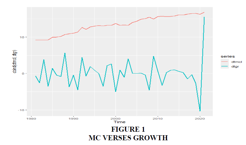
A cointegration time series technique has used the correlation between several time series analyses in the long term. This concept was introduced in 1987 by Robert Engle and Clive Granger, British economists. This test is for non-stationary data integrated as stationary from equilibrium in the long run. Before this tool, many researchers used linear regression to find the relationship between the variable for time series data. According to the authors, the relationship between the variable through stationarity and non-stationary data is good to get a significant value. There are two methods are there are cointegration techniques. I took Engle-Granger Two-Step Method. According to the Augmented Dickey-Fuller Test (ADF) used for the stationarity of the residuals. This study fails to reject the null hypothesis because the ‘p-value is 0.15. It is higher than the 0.05 cointegration between market capitalization and GDP. In this way, find the cointegration between central and state government securities, but there is no relationship between the security in times series data. The ‘p-value is 0.1233, which is higher than 0.05. It fails to reject the null hypothesis (Figure 1).

Hypothesis 1: MC vs Growth

NH: No Co-integration of mc with growth

AH: Co-integration of mc with growth exists.

> dtmc

Time Series:

Start = 1981

End = 2021

Frequency = 1

[1] 9769 9769 9769 10219 20378 21636 25937 45519 54560 65206 90836 323363 188146 368071 435481 526476 463915 560325

[19] 545361 912842 571553 612224 572198 1201207 1698428 3022191 3545041 5138015 3086076 6165620 6839084 6214912 6387887 7415296 10149290 9475328

[37] 12154525 14224997 15108711 11348757 20430815

> dtgr<-ts(dt$growth)

> dtgr<-ts(dt$growth)

> dtgr

Time Series:

Start = 1981

End = 2021

Frequency = 1

[1] -0.73 -2.53 3.81 -3.47 1.43 -0.48 -0.81 5.66 -3.68 -0.41 -4.48 4.43 -0.73 1.91 0.92 -0.02 -3.50 2.13 2.66 -5.00 0.98 -1.02 4.06

[24] 0.06 0.00 0.14 -0.40 -4.57 4.78 0.64 -3.26 0.22 0.93 1.02 0.59 0.26 -1.46 -0.34 -2.72 -10.33 15.54

> dtmcl<-log(dtmc)

> dtmcl

Time Series:

Start = 1981

End = 2021

Frequency = 1

[1] 9.186969 9.186969 9.186969 9.232004 9.922211 9.982114 10.163426 10.725885 10.907056 11.085307 11.416811 12.686531 12.144974 12.816031 12.984206 13.173961

[17] 13.047457 13.236272 13.209203 13.724318 13.256112 13.324854 13.257240 13.998837 14.345214 14.921493 15.081060 15.452177 14.942411 15.634499 15.738164 15.642462

[33] 15.669914 15.819055 16.132914 16.064202 16.313212 16.470511 16.530782 16.244619 16.832555

> dt1<-cbind(dtmcl,dtgr)

> head(dt1)

Time Series:

Start = 1981

End = 1986

Frequency = 1

dtmcl dtgr

1981 9.186969 -0.73

1982 9.186969 -2.53

1983 9.186969 3.81

1984 9.232004 -3.47

1985 9.922211 1.43

1986 9.982114 -0.48

Let us perform Co-integration test on this data.

> res

Phillips-Ouliaris Cointegration Test

data: dt1

Phillips-Ouliaris demeaned = -1.4088, Truncation lag parameter = 0, p-value = 0.15

Warning Message

In po.test(dt1): p-value greater than printed p-value

As the p-value is 0.15 > 0.05, fails to reject the NH, which means No Cointegration between MC and the Growth of the Economy.

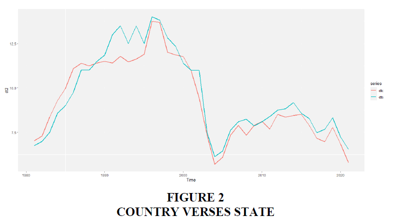
Hypothesis 2: Country vs State

NH: No Co-integration between the Country and state momentum.

AH: Co-integration exists between the Country and State Momentum (Figure 2).

> dtc

Time Series:

Start = 1981

End = 2021

Frequency = 1

[1] 7.03 7.29 8.36 9.29 9.98 11.08 11.38 11.25 11.40 11.49 11.41 11.78 11.46 11.63 11.90 13.75 13.69 12.01 11.86 11.77 10.95 9.44 7.34 5.71 6.11 7.34 7.89

[28] 7.34 7.89 8.12 7.69 8.52 8.36 8.45 8.51 7.89 7.16 6.97 7.78 6.85 5.80

> dts<-ts(dt$state,start=1981)

> dts

Time Series:

Start = 1981

End = 2021

Frequency = 1

[1] 6.75 7.00 7.50 8.58 9.00 9.75 11.00 11.00 11.50 11.84 13.00 13.50 12.50 13.50 12.50 14.00 13.82 12.82 12.35 11.39 10.99 10.99 7.49 6.13 6.45 7.63 8.10

[28] 8.25 7.87 8.11 8.39 8.75 8.84 9.18 8.58 8.28 7.48 7.67 8.32 7.24 6.55

> dt2<-cbind(dtc,dts)

> head(dt2)

Time Series:

Start = 1981

End = 1986

Frequency = 1

dtc dts

1981 7.03 6.75

1982 7.29 7.00

1983 8.36 7.50

1984 9.29 8.58

1985 9.98 9.00

1986 11.08 9.75

> autoplot(dt2)

> autoplot(dt2, lwd=1)

> po.test(dt2)

Phillips-Ouliaris Cointegration Test

data: dt2

Phillips-Ouliaris demeaned = -16.006, Truncation lag parameter = 0, p-value = 0.1233

As the p-value is above 0.05, the study fails to reject the NH that there is no cointegration between country and state momentum, even though it seems to exist from the plot.

Auto-regression Integrated Moving Average Techniques.

For analyzing the data based on the statistical tool Auto Regression Integrated Moving Average from 1980-2022. It is one technique projecting future price sustainable development of the capital market. This model denotes (p, d, q) where p is the autoregressive model, d is the variation, and q is the moving average model. This model helps transform non-stationary into stationary ones based on past and future can forecast. This technique is used for subjectivity, long-term, and more complex, and it is not for seasonal time series. To build the Arima model based on trends and use autocorrelation to determine the order of regression and moving average. This model analyses and builds a forecasting model that represents a time series by modelling the correlations in the data (Bora, 2021). Auto-Regression: It is the lagged value of ‘y’, until p time in the past, as predictors. The constant value is ‘c’, and ‘0’ are parameters. Integrate I (d): The difference is taken as ‘d’ until the original series becomes stationary.

>dt=read.csv(file.choose())

> dtc=dtdt$MC

> dtc=dt$MC

> dtc

[1] 9769 9769 9769 10219 20378 21636 25937 45519 54560

[10] 65206 90836 323363 188146 368071 435481 526476 463915 560325

[19] 545361 912842 571553 612224 572198 1201207 1698428 3022191 3545041

[28] 5138015 3086076 6165620 6839084 6214912 6387887 7415296 10149290 9475328

[37] 12154525 14224997 15108711 11348757 20430815 26406501

> dts=(dtc,start=1980,frequency=1)

> dts=ts(dtc,start=1980,frequency=1)

> dts

Time Series:

Start = 1980

End = 2021

Frequency = 1

[1] 9769 9769 9769 10219 20378 21636 25937 45519 54560

[10] 65206 90836 323363 188146 368071 435481 526476 463915 560325

[19] 545361 912842 571553 612224 572198 1201207 1698428 3022191 3545041

[28] 5138015 3086076 6165620 6839084 6214912 6387887 7415296 10149290 9475328

[37] 12154525 14224997 15108711 11348757 20430815 26406501

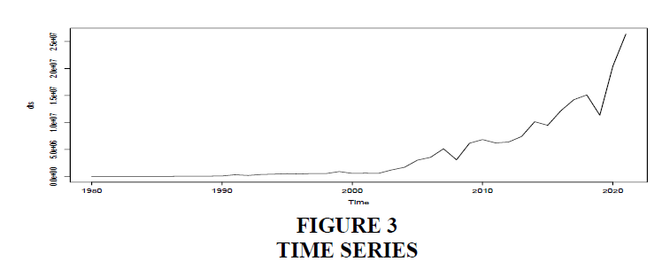
> plot(dts) (Figure 3)

>library(tseries)

> library(forecast)

> adf.test(dts)

Augmented Dickey-Fuller Test

data: dts

Dickey-Fuller = 3.9199, Lag order = 3, p-value = 0.99

alternative hypothesis: stationary

> #adf.test the Null Hypothesis (NH) not stationary and alternative hypothesis is stationary

> # kps.test() against the adf.test()

> kpss.test(dts)

KPSS Test for Level Stationarity

data: dts

KPSS Level = 0.93442, Truncation lag parameter = 3, p-value = 0.01

Warning message:

In kpss.test(dts) : p-value smaller than printed p-value

> auto.arima(dts,trace=T)

ARIMA(2,2,2) : Inf

ARIMA(0,2,0) : 1298.155

ARIMA(1,2,0) : 1287.058

ARIMA(0,2,1) : 1277.935

ARIMA(1,2,1) : 1279.872

ARIMA(0,2,2) : 1276.49

ARIMA(1,2,2) : Inf

ARIMA(0,2,3) : Inf

ARIMA (1,2,3) : In

Best model: ARIMA (0,2,2)

Series: dts

ARIMA(0,2,2)

Coefficients:

ma1 ma2

-1.5877 0.8608

s.e. 0.1200 0.1481

sigma^2 = 3.414e+12: log likelihood = -634.91

AIC=1275.82 AICc=1276.49 BIC=1280.89

> # Best model: ARIMA(0,2,2)

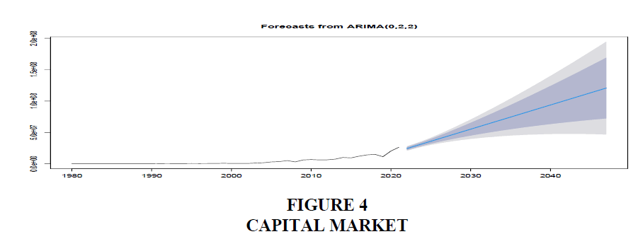
> fit=arima(dts,order=c(0,2,2))

> fit

Call:

arima(x = dts, order = c(0, 2, 2))

Coefficients:

ma1 ma2

-1.5877 0.8608

s.e. 0.1200 0.1481

sigma^2 estimated as 3.244e+12: log likelihood = -634.91, aic = 1275.82

> dtsf

Point Forecast Lo 80 Hi 80 Lo 95 Hi 95

2022 24385609 22076988 26694229 20854878 27916339

2023 28238292 25740754 30735830 24418637 32057947

2024 32090976 29133816 35048135 27568390 36613561

2025 35943659 32249629 39637689 30294128 41593191

2026 39796343 35134182 44458503 32666184 46926502

2027 43649027 37834452 49463601 34756402 52541652

2028 47501710 40384033 54619387 36616162 58387258

2029 51354394 42805317 59903471 38279708 64429079

2030 55207077 45113500 65300655 39770283 70643872

2031 59059761 47319364 70800158 41104373 77015149

2032 62912445 49430922 76393967 42294236 83530653

2033 66765128 51454391 82075865 43349377 90180880

2034 70617812 53394761 87840862 44277429 96958195

2035 74470495 55256160 93684831 45084705 103856286

2036 78323179 57042080 99604278 45776547 110869811

2037 82175863 58755535 105596190 46357563 117994163

2038 86028546 60399163 111657929 46831788 125225305

2039 89881230 61975306 117787154 47202802 132559657

2040 93733913 63486062 123981765 47473816 139994011

2041 97586597 64933328 130239866 47647732 147525462

2042 101439281 66318835 136559727 47727194 155151368

2043 105291964 67644167 142939762 47714627 162869302

2044 109144648 68910786 149378509 47612267 170677029

2045 112997331 70120048 155874614 47422186 178572477

2046 116850015 71273213 162426817 47146311 186553719

2047 120702699 72371457 169033941 46786443 194618955

> plot(dtsf)

> accuracy(dtsf)

ME RMSE MAE MPE MAPE MASE ACF1

Training set 335421.7 1757596 938154.2 6.510488 23.73524 0.9200913 0.1297428 (Figure 4)

Recommendations

From the above analysis is recommended that there is no relationship between the capital market and the development of an economy. The performance of yield on government securities state and central, there was no cointegration in the last forty years. But both the securities paid the highest yield rate during 1986-02 from 9.75% to 14.00%. In the last forty years, the low coupon rate paid by both securities is 5.50%. From the data in 1986-88, the capital market increased from 25937 crores to 45519, and the GDP raised to 9.63 from 3.97. In 1989-90 the capital market increased from 65206 crores to 90836 crores, but the GDP showed a negative growth rate of -4.48, reduced from 5.53 to 1.06. Recently, the capital market increased from 1,13,48,757 to 20430815, and in 2019-21 the GDP increased from 6.60% to 8.95%. It recommended that GDP does not measure the stock market GDP measures government spending, personal consumption net exports and also recommend that the GDP does have no impact on the stock market and that investors are optimistic about the future economy. The development of the economy has influenced various sectors of consumption and investments. Some exogenous factors that effects the economy are current government policies, decisions on households and companies for their provision of human capital and the formation of capital for productive purposes (Romer, 1986). At the bottom line, the stock market creates optimism for consumers, investors and businesses. From the capital market point of view, it recommended a positive outlook for the investors in the future to predict the capital market would be raising 19,46,18,955 crores by the coming independence year. It indicates a positive outcome for the investors to mobilize their resources in the capital market for the sustainable development of an economy.

Conclusion

In the global, India’s capital market is significant. India’s economy is growing, but at the same time, some problems and obstacles are faced due to the formation of capital in internal or international markets. Liberalization in the capital market helps improve the functioning of the stock market. At the same time, several internal and external factors and unforeseen factors played an adverse effect on the capital market. Revamp the regulations required for derivative products for risk management in the capital market. The primary and secondary markets should strengthen with international standards. Development of the debt market, especially in the corporate is essential for providing considerable assurance to bond investors.

References

Boesler, M. (2013). The economist who invented the BRICs just invented a whole new group of countries: the MINTs. Business Insider, 13.

Google Scholar

Carlin, W., & Mayer, C. (2003). Finance, investment, and growth. Journal of financial Economics, 69(1), 191-226.

Indexed at, Google Scholar, Cross Ref

Eichengreen, B. (2006). Asian bond market: Issues and prospects. Monetary and Economic Department.

Indexed at, Cross Ref

Greenwood, J., & Jovanovic, B. (1990). Financial development, growth, and the distribution of income. Journal of political Economy, 98(5, Part 1), 1076-1107.

Indexed at, Google Scholar, Cross Ref

Levine, R. (2003). More on finance and growth: more finance, more growth?. Review-Federal Reserve Bank of Saint Louis, 85(4), 31-46.

Indexed at, Google Scholar, Cross Ref

Patil, R. H. (2006). Current State of the Indian Capital Market. Economic and Political Weekly, 1001-1011.

Google Scholar

Rajan, R.G., & Zingales, L. (1998). Which capitalism? Lessons form the east Asian crisis. Journal of applied corporate finance, 11(3), 40-48.

Indexed at, Google Scholar, Cross Ref

Romer, P.M. (1986). Increasing returns and long-run growth. Journal of political economy, 94(5), 1002-1037.

Indexed at, Google Scholar, Cross Ref

Sakakibara, E. (2001, July). The East Asian Crisis-Two Years Later. In Annual World Bank Conference on Development Economics 2000 (pp. 243-255). World Bank Publications.

Indexed at, Google Scholar

Singh, A. (1997). Financial liberalisation, stockmarkets and economic development. The economic journal, 107(442), 771-782.

Indexed at, Google Scholar, Cross Ref

Smith, T.A., & Rajan, A. (2017). A Regression Model to Predict Stock Market Mega Movements and/or Volatility Using Both Macroeconomic Indicators & Fed Bank Variables. International Journal of Mathematics Trends and Technology, 49(3), 165.

Indexed at, Google Scholar

Takagi, H. (2001). Interactive evolutionary computation: Fusion of the capabilities of EC optimization and human evaluation. Proceedings of the IEEE, 89(9), 1275-1296.

Indexed at, Google Scholar, Cross Ref

Zegada Escobar, A.S. (2011). Capital market development and economic growth in Bolivia (Master's thesis, University of Twente).

Google Scholar

Received: 07-Feb-2023, Manuscript No. AMSJ-23-13206; Editor assigned: 08-Feb-2023, PreQC No. AMSJ-23-13206(PQ); Reviewed: 28-Mar-2023, QC No. AMSJ-23-13206; Revised: 22-Apr-2023, Manuscript No. AMSJ-23-13206(R); Published: 22-May-2023