Introduction

For the last few years, the focus of monetary policy has been shifted from direct monetary dynamics of real activity to other related associations between monetary policy and real activity. One of these relations that received considerable popularity is the sectoral effects of monetary policy. Additional and important information can be gathered by looking at the reaction sector-wise loan supply towards monetary shocks and assessing its impact on various sectors of the economy. Information from this approach may unfold some grey areas that can enhance the monetary policy's effectiveness.

A standard agreement prevails among economists that monetary policy works through the interest rates because an increase or decrease in interest rate leads to a reduction or expansion of interest-sensitive sectors of the economy. Our goal while covering this aspect is to oversee the disaggregated effect of monetary transmission in Pakistan. Suppose broken into various segments whether sectoal loan supply brings similar responses towards monetary shocks. These segments represent different economic sectors, e.g. loan is supplied to agriculture, manufacturing, consumer, services, trade and commerce sectors of the economy.

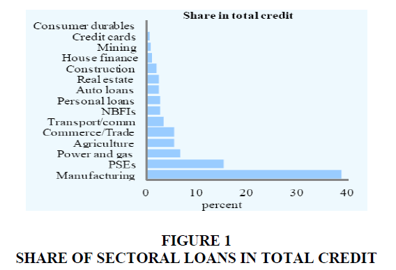
Figure 1 shows the sector-wise loan supply where the more significant portion is supplied to the manufacturing sector, followed by Public Sector Enterprises (PSE).

Various studies advocate the idea of varying effects of sectoral responses during monetary transmission. Monetary policy can have adverse effects at the aggregate level. However, some sectors react differently with varying magnitude(Ganley & Salmon, 1997), (Hayo & Uhlenbrock, 1999) (Serju, 2003).

Some examples are quoted here to present an overview of how sectors respond during monetary transmission; for instance, the construction sector performed more sensitively towards monetary shocks, followed by the manufacturing, services and agriculture sector in the Euro area(Ganley & Salmon, 1997). Another study also revealed that heavy industries react more impulsively than those producing consumer items such as clothing and food(Hayo & Uhlenbrock, 1999). Commercial and industrial loans respond more strongly than total loans portfolios to monetary shock. Industrial loans in developed countries are acquired by large corporate reacts more strongly than any other form of business toward monetary tightening (Gertler & Gilchrist, 1993; Kashyap & Stein, 1995).

It varies from economy to economy whether sectors react aggressively towards monetary shock. For instance, individual firm-level data gathered in a study reveals that financial constraints cause firms to respond more strongly, wherein small firms respond more strongly than more prominent firms because smaller firms are found to be more dependent on bank loans by their liquidity problems and small revenues (Kashyap & Stein, 1994).

Studies from developing countries reveal that agriculture and manufacturing sectors are negatively associated with monetary tightening. Sometimes it causes a deep recession because these sectors are the primary engines of developing economies(Serju, 2003). The above discussion supports the idea of unwinding important information by focusing on the sectoral response of loans, i.e. manufacturing, agriculture, trade and commerce, services and consumer sectors. Commercial banks in Pakistan holds a dominant position and constitutes the largest share of the total financial assets of Pakistan. In Pakistan, most studies focused on the responses at the aggregate level, however, this study will bring sectoral responses rarely studied by using disaggregated data.

Monetary tightening can have moderate effects from an aggregate perspective; however, it may have severe effects from a sector-specific point of view. From this disaggregated approach, a few studies have been conducted in the recent past that revealed that loan supply to various sectors of the economy responds heterogeneously in response to monetary shocks. Hence, monetary policy may have substantial distributional effects triggered by sector-specific monetary policy. Whether a particular sector responds quickly and aggressively toward monetary shocks to other sectors, Sectoral responses may provide valuable information. In Pakistan, sectoral responses need to be unfolded to add sector-specific monetary aspects while formulating monetary policy. So the question arises what will be the impact of the monetary policy rate on each sector of bank loans (i.e. manufacturing, agriculture, trade and commerce, services and consumer)?.

We state our research hypotheses as follows

H₁. An increase in monetary policy rates leads to a decrease in sectoral components of bank loans. (Negative)

a. An increase in monetary policy rate is negatively associated with advances in the manufacturing sector

b. An increase in monetary policy rate is negatively associated with advances in the consumer sector

c. An increase in monetary policy rate is negatively associated with advances in the services sector

d. An increase in monetary policy rate is negatively associated with advances in the trade and commerce sector

e. An increase in monetary policy rate is negatively associated with advances in the agriculture sector

Review of Literature

Most of the studies are conducted on monetary transmission using aggregated data; however, limited studies are witnessed exploring essential aspects of monetary transmission at a disaggregate level, especially in Pakistan. Previously we discussed the association of loan supply with policy changes; however, how policy variable affects components of loans given to various sectors of an economy entails significant information.

Various studies were conducted in the past unfolding relationship between monetary shocks and sectoral performance of banks loans. Multiple studies confirm varying effects of monetary shocks on components of banks loans. For instance, an analysis detected that sectoral portfolios of bank loans worked differently than the total portfolio of bank loans by using VAR (Bernanke & Gertler, 1995). These sectors or components of bank loans are based on the nature of activity a particular industry performs during monetary transmission. For example, suppose an economy is divided into several sectors, i.e. agriculture, manufacturing, trade and commerce, consumers, and services. In that case, each sector’s loan supply may show a varying response to the total collection of bank loans after receiving monetary shocks.

Some other studies also endorse sectoral responses to bank loans in that commercial and industrial loans respond more strongly than the portfolio of total loans after a monetary shock (Gertler & Gilchrist, 1993; Kashyap & Stein, 1995). Similarly, a study also utilized disaggregated credit supply data, including consumer and real estate lending, revealing varying effects. This study revealed that access to non-bank credit sources in the real estate and consumer goods sector impedes effective monetary transmission. Further, extensive securitization of reals sector and consumer finance loans makes it difficult for small businesses to avail these lending facilities because of the varying effects of such loans in a monetary transmission (Morris & Sellon Jr, 1995).

Other sectors, such as loan supply to individuals, usually called consumer loans, could not be affected by monetary shocks even though if total supply of loans is significantly affected. For instance, credit card loans could not be affected by the monetary shocks due to an individual's short-term dire necessities. This study compiled monthly data from 1989 to 1991 from USA banking institutions where the prime rate dropped from 11.5 per cent to 7.5 per cent; however, no considerable change was passed through to the largest issuers of credit cards which remained fixed at 18 to 20 per cent. Therefore, surprisingly no significant response is detected in the loan supply of credit card loans (Calem & Mester, 1995).

A study revealed that the durability of goods also counted in varying effects of sectoral loan supply because those firms manufacture durable items that could not insulate monetary shocks. Germany's industrial data revealed that heavy industries in the manufacturing sector react more strongly toward monetary shocks than those producing non-durable items such as clothing and food being basic consumer necessities(Hayo & Uhlenbrock, 1999).

Similarly, another study witnessed Commercial and Industrial (C&I) loans increase, whereas total bank lending reduced after a monetary tightening. This study witnessed an increase in C&I loans due to a reduction in real activity. It is also examined that the bank lending channel exists only concerning the USA’s consumer and real estate loans. Inventories display a temporary increase followed by a decline; however, no evidence of the rise in stocks caused by the increase in C&I loans (Haan, Sumner, & Yamashiro, 2009).

Another aspect that emphasizes varying effects is the approval structure of banking loans, particularly when a loan is sanctioned to a specific borrower group. For instance, business loans are not made under terms of the loan commitment, and these loans would appear most vulnerable to monetary shocks because banks may change their other loan approval process with the change in monetary stance. However, the loans provided under the existing loan commitment remained unaffected (Sofianos, Wachtel, & Melnik, 1990).

Another study examined the same aspect by studying the balance sheets of banks. This study concluded that bank loans represented by the smallest asset category on the balance sheet of various banks responded more aggressively to monetary shocks (Kashyap & Stein, 1995). Likewise, a study also supported the same idea as an increase in the securitisation of loans weakened the efficacy of bank lending channels. This study used banking data of various European banks (Altunbas, Gambacorta, & Marques-Ibanez, 2009).

Intercountry varying effects of corporate loans were detected by a study that compared ratios of total assets of the banks to GDP of the four largest European economies with the USA. This study revealed that corporate loaning in Europe relies more significantly on banks while the corporate sector of Europe relies more on bank financings than the USA. However, some differences were also prevailing at the country level; for instance, French firms are debt-financed ten times more than the Italian firms. Similarly, loans are matured early in Italy than in France. Such early maturities are likely to speed up the monetary transmission since loans can be refinanced more frequently (Monticelli & Tristani, 1999).

Varying effects of the sectoral loans are also based on firm capacities as how firms operate and what challenges a firm encounters in a particular sector to germinate a variable response. A study analysed that external funds are more expansive to raise than funds are raised internally. Therefore, those firms that depend more on external financing are likely to be affected more by monetary tightening. It is also witnessed that non-bank loans could not easily replace bank loans; therefore, stock prices of those firms increased, which announced loan agreements with banks (James, 1987).

Likewise, those firms unable to find other sources of external finance witnessed varying effects based on their size. Small and medium enterprise firms are more responsive to monetary policy changes than large firms because large firms have better liquidity to insulate monetary shocks (Gertler & Gilchrist, 1993). Individual firm-level data also revealed that a firm's financial constraints during monetary tightening might cause small firms to react more (Kashyap & Stein, 1994) (Gertler & Gilchrist, 1994). On the same line, a study investigated that small firms are less accessible to the bank or non-bank external finance during monetary tightening(Oliner & Rudebusch, 1996). These firm-level restrictions and limitations develop varying effects on bank loans in various sectors if surrounded by firm-level uniformity or non-uniformity.

The above literature review validates varying effects of sectoral loan supply in monetary transmission based on firm-level limitations and restrictions in the market, e.g. nature of product or services a firm deals with or firm's size, capacity or financials. Every firm in the market stands differently and reacts differently to changing market dynamics. Therefore studying different sectors of the economy and how they respond to monetary shocks entail significant information. However, rarely any study in Pakistan is conducted which unfolds these differences. These differences may depend on various factors, such as loan demand, securitisation a firm holds to obtain a loan, debt benefit, particular focus and government subsidy a firm enjoys. In this study, the disaggregated level data of sectoral loans of Pakistan are investigated.

Research Methodology

This study focuses on sectoral forms of entire bank lending, divided into five broader categories, i.e. Agriculture, manufacturing, commerce and trade, services and consumer loans. Advances in the above segments are categorized as agriculture, which comprises growing crops, farming of animals, agriculture and animal husbandry services, agriculture machinery and equipment, hunting, trapping, forestry and logging, etc.

Whereas the manufacturing sector encompasses all the loans given to the textile sector, including all textile functions, food products and beverages, tobacco products, wood and products of wood, paper, paper board, printing, publishing and allied industries, coke refined petroleum products, chemicals, rubbers and plastics products, metals, machinery and equipment, electrical machinery and related apparatus, medical, precision and optical instruments, watches and clocks, Motor vehicles and related industries, furniture and fixtures, jewellery and related articles, sports and handicrafts industries etc.

Similarly, the commerce and Trade sector is divided into the sale, maintenance and repair of motor vehicles, whole sale retail trade, and commission trade, including exports, imports, and domestic wholesale. Likewise, credit supplied in the Services sector includes the credit supplied to hotels and related industries, Transport, communication, real estate business activities, education and health and social work etc. Last but not most minor consumer sector consists of all the loans granted for house building, purchase of cars, consumer durables, credit cards and personal loans.

After going through the data dynamics, It is revealed that the agriculture lending varies approximately from 5 per cent to 8 per cent of the total advances, manufacturing 50 per cent to 62 per cent, commerce and trade 7 per cent to 10 per cent, Services from 9 per cent to 15 per cent and consumer financing from 5 per cent to 15 per cent of the total advances during 2006 to 2018 (Banking performance report www.sbp.org.pk).

KIBOR is used as a proxy of monetary shocks, which we have discussed earlier as an Independent variable, whereas sectoral loan supply is used as the dependent variable of our study. Quarterly data in log form of commercial banks operating in Pakistan is taken from June 2006 to March 2018 (Table 1).

Table 1 Conceptual/Theoretical Framework
Impact of Monetary Policy on Sectoral Bank Loans	Dependent Variables	Relationship	Code	Independent Variables	Sources	Econometric Model used by various Authors
	Commence and Trade Finance		CT	KIBOR	(Algan & Ragot, 2010) (Sukmana & Kassim, 2010) (Arestis & Sawyer, 2006), (Gertler & Gilchrist, 1993; Kashyap & Stein, 1995),(Morris & Sellon Jr, 1995), (Calem & Mester, 1995), (Monticelli & Tristani, 1999), (James, 1987), (Gertler & Gilchrist, 1993), (Kashyap & Stein, 1994),(Gertler & Gilchrist, 1994), (Oliner & Rudebusch, 1996)	VAR (Hayo & Uhlenbrock, 1999), VAR , JJ Co-integration (Haan et al., 2009), VAR, VECM(Sofianos et al., 1990), VAR, ECM (Kashyap & Stein, 1995), VECM (Altunbas et al., 2009)
	Agriculture Finance		AGR
	Consumer Finance		CONS
	Manufacturing Finance		MANF
	Services Finance		SERV
	Total Advances		TA
			KBR
	Consumer Price index		CPI
	Industrial Product Index		IPI

The data for this research is collected from the published sources of the State Bank of Pakistan; therefore, no permissions will be required to collect data other than the respondents' informed consent.

Unit root tests are employed whether a variable is not stationary and possesses a unit root where the null hypothesis identifies the presence of a unit root and the alternative hypothesis shows stationarity. The Augmented Dickey-Fuller (ADF) test will be employed to check Unit roots. The T statistics of ADF results are more significant than the values at a 5 or 10 % significance level at the first difference. The lag length determination test is beneficial to avoid autocorrelation (Fuller, 1976).

The data gathered from designated sources will then be analyzed and evaluated to investigate the effectiveness of various banking channels in monetary transmission by using statistical software like Microsoft Excel and E-views. The research intends to exploit Regression through VAR, VECM, IRF, VDA. A model in equational form defines every hypothesis in our analysis. In addition, impact variables were compared to examine and evaluate cross-sectional differences.

We employ the Vector Autoregression VAR methodology developed by Sims in 1980, which assumed that all variables in the model are endogenous therefore called a non-theoretical model. This study examines the effects of monetary shocks on real output and prices. Prominent empirical literature witnesses the utilization of the VAR approach based on variance decomposition analysis and impulse response functions to examine the effect of credit channel on critical economic variables, i.e. output and inflation(Agha, Ahmed, Mubarik, & Shah, 2005; Baig; Bernanke & Blinder, 1992; Hussain, Berg, & Aiyar, 2009).

The impulse response function indicates how the economy reacts with time's passage to exogenous impulses, also called shocks used in a VAR system. Impulses taken in the exogenous form include policy shocks in the shape of change in monetary tools, e.g. policy rate or interest rate. The impulse response function detects the reaction of endogenous macroeconomic variables, e.g., output and prices, at the time of shock, and subsequently, the shock is passed. Since our focus in this study is to interpret the monetary shock on real output, we drive an impulse response function that traces real output's reaction at one standard deviation shock to the interest rate.

To know the proportion of fluctuations of given variables passed through different shocks in the VAR system can be examined through variance decomposition. First, it reveals the fraction of forecast variance error of the variables caused by their shocks versus shocks of endogenous variables. In simple words, VAR is a stochastic process used to detect the linear interdependencies among multiple time series. All variable in VAR is included altogether so that each variable acquire an equation explaining its evolution that is derived from its own lagged value. In VAR, endogenous variables in the system are functions of lagged values of all endogenous variables. VAR is identified by using Cholesky decomposition, which further used recursive orthogonalization to isolate the underlying structure with the innovation of the first equation untransformed the innovation in the second equation taken as orthogonal to the first one so on.

An essential issue in VAR estimation is to use the appropriate strategy in the specification of the VAR, whether VAR should be estimated in pure differences or levels without the imposition of any restriction or with restriction usually known as Vector Error Correction Model VECM to allow the presence of co-integration. It depends on the data properties, i.e. unit root and co-integration. If the variables in a VAR are found non-stationary and are not co-integrated, then VAR should be specified in pure differences. While estimating the VARs where some variables are non-stationary does not affect the estimator consistency. Instead, it affects efficiency by being non-stationary, as referred to by Sims 1980 (Sims, Stock, & Watson, 1990).

However, the objective of VAR is to determine the relationship among variables rather than to concentrate on efficiency. Contrarily, if the variables are integrated of the same order and co-integrated, VECM is the preferred specification since it can generate efficient estimates without losing information for the long-run relationship among the variables. Many researchers suggested against simply looking at the statistical properties of the data to decide on appropriate specification Ramaswamy and Slok (1998).

VECM is estimated if co-integration exists, and if co-integration does not exist, then imposing co-integration may not be an appropriate estimation strategy. Imposing inappropriate co-integration relationships can lead to biased estimates and result in a biased impulse response derived from the reduced form of VAR. Consequently, unrestricted VAR with a difference will be estimated if no co-integration exists and variables are stationary at first.

ECM and VECM techniques will be employed to detect short term dynamics and speed of adjustment(Sims, 1980). VECM is the preferred specification since it can generate efficient estimates without losing information for the long-run relationship among the variables. However, many researchers suggested against simply looking at the statistical properties of the data to decide on appropriate specifications (Ramaswamy & Slok, 1998).

To clarify the results, Impulse Response Functions (IRF) will be derived from Vector Error Correction Model (VECM) to determine the short-run pass through the response of policy rate on deposit rate and lending rate. An impulse response function has paramount importance to elaborate multivariate linear models by presenting measures of statistical reliability. All the models are classified on two bases. Firstly according to the magnitude of the responses with less than 1 per cent decline in deposit or lending rate (relative to the baseline) to one standard deviation shock of policy rate and similarly with greater than 1 per cent. Secondly, according to the duration of the responses wherein decline in deposit and lending rate bottoms out within a specified period and those wherein deposit and lending rate decline bottoms out after that period.

After going through the impulse response dynamics, the subsequent analysis that can further assess our study objectives is variance decomposition. It indicates how much information is contributed by each variable to other variables in an autoregression and how much the exogenous shock of other variables can elaborate forecast error variance of each variable. For example, the value of a variable forecasted from its own lagged values will have all its forecasted error variance accounted for by its disturbances and explain all its forecast error variance at short horizons and a little at longer horizons. Various impulse responses are shown in graphical form, and variance decomposition tables are computed in tabular form. A model in equational form defines every hypothesis in our analysis. Impact variables were compared in order to examine and evaluate cross-sectional differences.

The following VAR model is identified as follows equation 1 (Den Haan, 2000)

Here X_t is a vector of variables, t represents time trend, and L is the lag dimension of the VAR. It involves estimating the above equitation and obtaining values for K-period forecasts for variables in X_t and later evaluating K-period forecast errors, net of actual values X_t and in-sample forecast values. The minimum number of lags will be restricted to two using Schwarz’s Bayesian information criterion, which helps us preserve data length.

VAR parsimonious four variables of interest used by using the widely used recursive identification scheme in which two macro-economic variables, i.e. real output represented by Industrial Production Index (IPI) and prices represented by Consumer Price Incex (CPI) are used with the policy variable, i.e. R placed last in Cholesky order, and bank loans B i.e. loans granted in various sectors affecting these macroeconomic variables with a lag (Bernanke & Blinder, 1992). X_t matrix in the above model will be as follows. T denotes a time trend, and L is a lag dimension of the VAR.

X _t = [IPICPIBR]

Since the focus is to identify the bank lending channel, VAR will also be employed on disaggregated data. For this purpose, we used data of credit supplied to five sectors representing part of economy banks. Hence in total various VARs will be estimated

Lending Channels

a .IPI, CPI, Total Loans, KIBOR

b. IPI, CPI, Manufacturing Loans, KIBOR

c. IPI, CPI, Agriculture Loans, KIBOR

d. IPI, CPI, Commerce and Trade Loans, KIBOR

e. IPI, CPI, Services Loans, KIBOR

f. IPI, CPI, Consumer Loans, KIBOR

Estimation and Inferences

The first step in our estimation of data dynamics is to employ a Unit root test to detect the stationary of the data, whether data is stationary at level or first difference. Next, the impulse response function (IRF) will be used to detect a response of a given variable at 1 per cent or 100 basis points (bps) standard deviation shock with other variables in the model. Finally, variance Decomposition analysis will be undertaken to analyze the relative contribution of a variable to explain the variability of its endogenous variables.

The Augmented Dickey-Fuller (ADF) and Phillips Perron (PP) tests were employed to check Unit roots. ‘T’ statistics of ADF and PP were more significant than the values at a 5 % significance level at the first difference, as shown. The lag length determination test is employed to avoid autocorrelation in the VAR system. It is considered that after utilization of lag optimum, there would not be any further autocorrelation exists in the system. The results in Table 2 show that the equation model has a lag optimum at lag 6.

Table 2 Lag Length Criteria
Lag	LogL	LR	FPE	AIC	SC	HQ
0	3304.234	NA	2.44e-33	-49.55239	-49.35680*	-49.47291*
1	3404.409	185.2859	1.83e-33	-49.84073	-47.88486	-49.04594
2	3492.149	150.4126	1.68e-33*	-49.94210*	-46.22593	-48.43199
3	3551.938	94.40236	2.41e-33	-49.62312	-44.14667	-47.39770
4	3609.988	83.80248	3.68e-33	-49.27802	-42.04128	-46.33728
5	3672.927	82.34114	5.51e-33	-49.00642	-40.00940	-45.35038
6	3798.915	147.7751*	3.44e-33	-49.68293	-38.92562	-45.31157
7	3887.216	91.62043	4.19e-33	-49.79272	-37.27512	-44.70604
8	3974.574	78.81948	5.92e-33	-49.88833	-35.61044	-44.08634

JJ (Johansen & Juselius, 1990) tests are used to find the maximum likelihood ratios or Cointegration to detect the long-run relationship among variables not detected during the integration process (Table 3). Trace statistics in Table 4 indicate that no co-integration rank exists at a 5% level of significance. The absence of co-integration allows the implementation of the VAR test with the difference (Ascarya, 2012).

Table 3 Unit Root Test
	ADF			Phillip Parren
		Level	1st Difference	Level	1st Difference
		t-Stat	t-Stat	Adj. t-Stat	Adj. t-Stat
Agriculture (AGR)		-1.78	-11.19	-1.92	-15.63
	1% level	-4.02	-4.03	-4.02	-4.02
	5% level	-3.44	-3.44	-3.44	-3.44
Consumer Loan Cons		-1.39	-4.61	0.65	-10.83
	1% level	-4.03	-4.03	-4.02	-4.02
	5% level	-3.44	-3.44	-3.44	-3.44
Consumer Price Index (CPI)		-2.68	-10.36	-2.60	-10.36
	1% level	-4.02	-4.02	-4.02	-4.02
	5% level	-3.44	-3.44	-3.44	-3.44
		-0.94	-11.40	-0.83	-11.56
Commerce and Trade (CT)	1% level	-4.02	-4.02	-4.02	-4.02
	5% level	-3.44	-3.44	-3.44	-3.44
		3.25	-7.97	1.19	-16.99
IPI	1% level	-4.03	-4.03	-4.02	-4.02
	5% level	-3.44	-3.44	-3.44	-3.44
		-2.76	-4.96	-2.40	-7.83
MANF	1% level	-4.03	-4.03	-4.02	-4.02
	5% level	-3.45	-3.45	-3.44	-3.44
SERV		-2.95	-13.81	-2.95	-14.53
	1% level	-4.02	-4.02	-4.02	-4.02
	5% level	-3.44	-3.44	-3.44	-3.44
		-1.64	-2.00	-1.42	-8.92
TA	1% level	-4.03	-4.03	-4.02	-4.02
	5% level	-3.45	-3.45	-3.44	-3.44
KBR		-0.58	-8.20	-0.74	-7.57
	1% level	-3.48	-3.48	-3.48	-3.48
	5% level	-2.88	-2.88	-2.88	-2.88

Table 4 Unrestricted Cointegration Rank Test (Trace)
Hypothesized		Trace	0.05
No. of CE(s)	Eigenvalue	Statistic	Critical Value	Prob.**
None	0.119217	41.78866	47.85613	0.1647
At most 1	0.094271	24.65115	29.79707	0.1743
At most 2	0.080023	11.28407	15.49471	0.1946
At most 3	0.000179	0.024182	3.841466	0.8763

Impulse Response Function and Variance Decomposition

VAR estimates for each sector are derived, and impulse responses are generated to evaluate sectoral performances. All five sectors are classified on two bases, firstly according to the magnitude of the responses and secondly, according to the duration of the responses. Hence, impulse response functions are derived from retrieving results. After that, the subsequent analysis that can add further clarity to our study objectives is variance decomposition analysis. It indicates how much information is contributed by each variable to other variables in autoregression and how the exogenous shock of other variables can elaborate much forecast error variance of each variable. The variable's value forecasted from its own lagged values will have all its forecasted error variance accounted for by its disturbances and explain its forecast error variance at short and long horizons. Results are shown in a graphical form derived through impulse responses and tabular forms derived through variance decomposition analysis.

Consumer Sector Financing

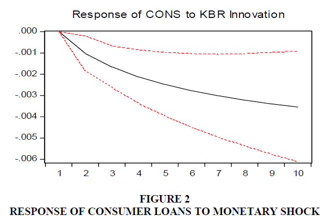
Figure 2 shows that the impulse response of loans supplied in the consumer finance sector declined below the baseline up to 30 bps after a 100 bps shock of KIBOR until the fifth month and remained on the opposing side. Table 5 shows that the 12 per cent forecasted KIBOR explains the error variance of consumer finance derived from variance decomposition until the end of the eighth month.

Table 5 Variance Decomposition Analysis of Sectoral Performance
Period	S.E.	D(CPI)	D(IPI)	D(SERV)	D(KBR)	Period	S.E.	D(IPI)	D(CPI)	D(KBR)	D(AGR)
1	0.07	0.06	0.64	99.31	0.00	1.00	0.03	0.03	2.49	0.01	97.47
2	0.07	0.06	0.87	99.03	0.03	2.00	0.03	0.66	3.37	1.56	94.42
3	0.07	0.12	0.99	97.04	1.86	3.00	0.04	0.77	4.34	3.20	91.69
4	0.07	2.31	1.10	94.76	1.83	4.00	0.04	1.56	4.31	3.56	90.57
5	0.07	2.38	2.04	93.34	2.24	5.00	0.04	1.79	6.73	4.01	87.46
6	0.07	2.32	2.00	92.85	2.83	6.00	0.04	1.88	6.76	4.22	87.15
7	0.07	2.95	2.06	92.21	2.78	7.00	0.04	2.26	6.53	4.08	87.13
8	0.07	3.29	2.05	91.65	3.01	8.00	0.04	2.44	6.49	4.02	87.05
Period	S.E.	D(CONS)	D(CPI)	D(IPI)	D(KBR)	Period	S.E.	D(CPI)	D(IPI)	D(KBR)	D(CT)
1	0.00	100.00	0.00	0.00	0.00	1.00	0.07	1.88	1.25	0.44	96.44
2	0.01	93.44	0.14	0.00	6.42	2.00	0.07	2.12	1.24	1.62	95.02
3	0.01	86.92	0.82	3.04	9.22	3.00	0.07	3.31	1.20	1.79	93.70
4	0.01	84.23	2.03	3.85	9.90	4.00	0.07	3.59	1.25	1.94	93.21
5	0.01	80.05	2.80	6.57	10.58	5.00	0.07	3.71	1.55	1.91	92.83
6	0.01	79.52	2.65	6.20	11.63	6.00	0.07	5.02	1.52	1.87	91.60
7	0.01	78.94	2.48	7.94	10.64	7.00	0.07	4.64	1.45	2.28	91.63
8	0.01	77.04	2.97	7.84	12.15	8.00	0.07	4.74	1.54	2.46	91.26
Period	S.E.	D(CPI)	D(IPI)	D(KBR)	D(MANF)	Period	S.E.	D(CPI)	D(IPI)	D(KBR)	D(TA)
1	0.07	3.33	2.36	0.07	94.24	1.00	0.07	4.70	3.15	0.01	92.14
2	0.07	6.83	2.94	0.84	89.40	2.00	0.07	6.94	3.82	0.47	88.77
3	0.07	10.66	2.80	0.79	85.75	3.00	0.07	8.97	4.51	0.59	85.93
4	0.07	11.95	3.81	2.36	81.87	4.00	0.07	10.20	5.70	1.05	83.05
5	0.07	11.58	4.99	5.46	77.97	5.00	0.07	9.95	6.03	2.74	81.28
6	0.07	11.00	4.91	5.18	78.91	6.00	0.07	9.52	6.16	2.47	81.85
7	0.07	10.82	4.95	5.12	79.12	7.00	0.07	9.43	6.10	2.58	81.89
8	0.07	10.89	5.09	5.08	78.94	8.00	0.07	9.50	6.29	2.58	81.63
Period	S.E.	D(CPI)	D(IPI)	D(KBR)	D(TA)	Period	S.E.	D(CPI)	D(IPI)	D(KBR)	D(TA)
1	0.07	100.00	0.00	0.00	0.00	1.00	0.07	0.79	99.21	0.00	0.00
2	0.07	99.33	0.08	0.51	0.08	2.00	0.07	0.90	93.75	0.59	4.76
3	0.07	95.87	0.41	3.43	0.29	3.00	0.07	1.23	93.49	0.95	4.33
4	0.07	95.45	0.40	3.72	0.42	4.00	0.07	1.41	92.19	1.42	4.98
5	0.07	94.90	0.43	4.24	0.42	5.00	0.07	1.82	91.74	1.44	5.00
6	0.07	94.30	0.60	4.58	0.52	6.00	0.07	1.75	88.87	2.72	6.66
7	0.07	93.10	0.63	5.48	0.79	7.00	0.07	2.62	87.02	3.16	7.20
8	0.07	93.01	0.64	5.54	0.82	8.00	0.07	2.88	86.74	3.18	7.20

Agriculture Sector Financing

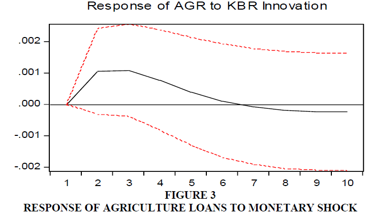
Figure 3 shows the impulse response of loans supplied in the agriculture sector after a 100 bps shock of KIBOR affects ten basis points until the third month. On the contrary, loans increased marginally after the shock and soon became stable after six months. Likewise, shows a weak contribution of 4 per cent forecasted KIBOR explains error variance of agriculture finance until the end of the eighth month.

Services Sector Financing

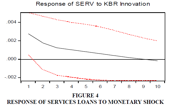
Figure 4 shows the output of services sector financing declining after a one standard deviation shock of interest rate, i.e. KIBOR could not influence service sector financing. On the other hand, results derived from variance decomposition, as shown, describe that interest rate contributed mildly to service sector financing, which was 3 per cent until the end of the eighth month.

Commerce and Trade Sector Financing

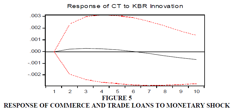
Figure 5 shows that commerce and trade sector financing output increases a little after a one standard deviation shock of interest rate, i.e. KIBOR means an increase in interest rate could not significantly influence commerce and trade sector financing. After increasing the monetary policy rate, the reaction remained less effective for the commerce and trade sector financing. Results derived from variance decomposition, as shown in Table 5, describe that interest rate contributed less significantly to commerce and trade sector financing, which was less than 3 per cent until the end of the eighth month.

Manufacturing Sector Financing

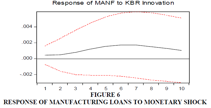
Figure 6 shows that the manufacturing sector's output increased for a shorter period and later stabilized after a one standard deviation interest rate shock, i.e. KIBOR means an increase in interest rate marginally influences the manufacturing sector. As shown in Table 5, results derived from variance decomposition describe that interest rate contributed less significantly to manufacturing finance, which was 5 per cent until the end of the eighth month.

Total Advances

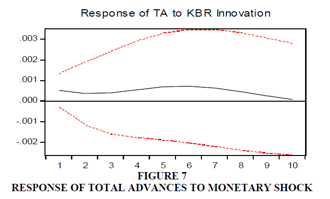
Figure 7 shows that the output of total credit supply is increased for a shorter period and later stabilized after a one standard deviation shock of interest rate, i.e. KIBOR. It means an increase in interest rate could not influence the total supply of loans. However, results derived from variance decomposition, as shown in Table 5, describe that interest rate contributed moderately to manufacturing finance, which was 2.5 per cent until the end of the eighth month.

Effects on Real Output

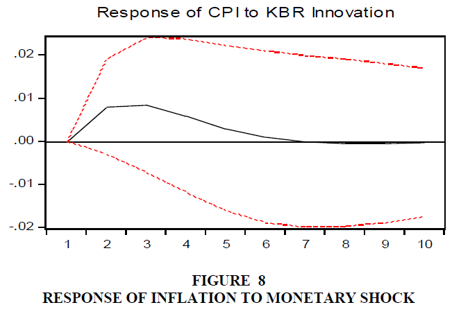
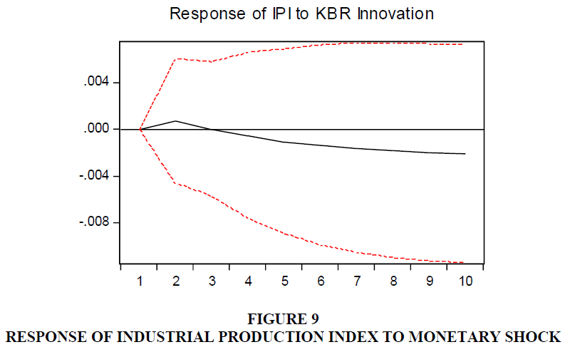
Figure 8 shows that the Output of the consumer price index and industrial production index is increased for a shorter period and later decreased either at the baseline or lower than that, respectively, after a one standard deviation positive shock of interest rate, i.e. KIBOR. It means an increase in interest rate could not influence real output significantly.

Results derived from variance decomposition analysis, as shown in Table 5, describe that interest rate contributed mildly to industrial production index, which is above 3 per cent till the end of the eighth month, whereas for consumer price index it is almost 5 per cent after the end of eight-month (Figure 9).

Concluding Remarks

This study assessed relationships between different sectoral loaning and monetary policy rates in a multivariate setting to determine whether monetary policy shocks have sectoral effects. Results of our assessment revealed a reduction in bank loans to consumers, whereas loans to the business side remain less effective. Consumer financing is found to be most responsive to the monetary policy rate. Lending to the agriculture and manufacturing sectors is moderately associated with the monetary policy rate. At the same time, the services, sector, trade, and commerce sectors showed a weak association with the monetary policy rate. Our results also support the idea which confirms that interest rates mainly stimulate consumption spending instead of business investment.

Consumer and agriculture financing is primarily associated with individuals, whereas the other sectors are linked with firm-level decisions. Firm-level financing decisions are associated with debt servicing costs because a consistent and sharp rise in interest rate increases debt servicing costs, affecting a firm’s financing decision to expand its operations and rely on bank loans exclusively. On the other side, some associated benefits a firm enjoys, i.e. advantage of using debt over equity and the tax benefit of encouraging firms to extend their financing needs even in case of monetary tightening.

Another aspect that hinders the growth of business loans in the SME sector of Pakistan is the prevalence of a high infection ratio. Share of the SME financing in total advances has varied from 5 to 10 per cent for many years even though SMEsconstitute nearly 90% of all the enterprises inPakistan. Likewise, the SME sector employs 80% of the non-agricultural labour force, and their share in the annual GDP is 40% approximately. Past data revealed that a high infection ratio, i.e. 17 %, was prevailing till the end of 2017, even reducing from 25 % in 2015. Similarly, Gross NPL to Loan Ratio (GNPLR) was roaming over 2 to 3per cent in 2008 and was increased to 15 % by the end of 2012. However, it was controlled and reduced to less than 6 per cent until the end of 2017.

The banks ignore the notably small and medium enterprises (SME) sector in Pakistan; therefore, the role of the SME sector is underperformed in real activity. The SME sector is the backbone of any economy. However, SBP needs to take appropriate steps to establish a sustainable SME sector in Pakistan. The role of lending channels in the business sectors may be strengthened, and SMEs may play a vital part in accelerating real activity.

This area of research can be used as a comparative study of various economies to jot down further factors influencing the sectoral performance of loans. Furthermore, studying varying effects of sectoral performance in the backdrop of monetary shocks is an important area from a policy point of view as monetary authorities in Pakistan can gauge their decisions by the impact of each sector.

References

Agha, A. I., Ahmed, N., Mubarik, Y. A., & Shah, H. (2005). Transmission mechanism of monetary policy in Pakistan. SBP-Research Bulletin, 1(1), 1-23.

Indexed at, Google Scholar

Arestis, P., & Sawyer, M. C. (2006). A handbook of alternative monetary economics: Edward Elgar Publishing.

Google Scholar

Ascarya, A. (2012). Transmission channel and effectiveness of dual monetary policy in Indonesia. Buletin Ekonomi Moneter dan Perbankan, 14(3), 269-298.

Indexed at, Google Scholar, Cross Ref

Bernanke, B. S., & Blinder, A. S. (1992). The federal funds rate and the channels of monetary transmission. The American economic review, 901-921.

Indexed at, Google Scholar, Cross Ref

Bernanke, B. S., & Gertler, M. (1995). Inside the black box: the credit channel of monetary policy transmission. Journal of Economic Perspectives, 9(4), 27-48.

Indexed at, Google Scholar, Cross Ref

Calem, P. S., & Mester, L. J. (1995). Consumer behavior and the stickiness of credit-card interest rates. The American economic review, 85(5), 1327-1336.

Indexed at, Google Scholar

Den Haan, W. J. (2000). The comovement between output and prices. Journal of Monetary economics, 46(1), 3-30.

Indexed at, Google Scholar

Fuller, W. A. (1976). Introduction to Statistical Time Series, New York: JohnWiley. FullerIntroduction to Statistical Time Series1976.

Google Scholar

Ganley, J., & Salmon, C. (1997). The industrial impact of monetary policy shocks: some stylised facts.

Indexed at, Google Scholar, Cross Ref

Haan, W. J. D., Sumner, S. W., & Yamashiro, G. M. (2009). Bank loan portfolios and the Canadian monetary transmission mechanism. Canadian Journal of Economics/Revue canadienne d'économique, 42(3), 1150-1175.

Google Scholar

James, C. (1987). Some evidence on the uniqueness of bank loans. Journal of financial economics, 19(2), 217-235.

Indexed at, Google Scholar, Cross Ref

Johansen, S., & Juselius, K. (1990). Maximum likelihood estimation and inference on cointegration—with applications to the demand for money. Oxford Bulletin of Economics and statistics, 52(2), 169-210.

Indexed at, Google Scholar, Cross Ref

Serju, P. (2003). Monetary policy and the Jamaican economy: a sectoral analysis. Research Service Department, Working Paper no. 02, 9.

Google Scholar

Sukmana, R., & Kassim, S. H. (2010). Roles of the Islamic banks in the monetary transmission process in Malaysia. International Journal of Islamic and Middle Eastern Finance and Management, 3(1), 7-19.

Indexed at, Google Scholar, Cross Ref

Received: 05-Oct-2024, Manuscript No. ASMJ-24-15316; Editor assigned: 07-Oct-2024, PreQC No. ASMJ-24-15316(PQ); Reviewed: 16- Oct-2024, QC No. ASMJ-24-15316; Revised: 25-Oct-2024, Manuscript No. ASMJ-24-15316(R); Published: 10-Nov-2024