Keywords

Song Popularity Prediction, Machine Learning in Music, Sentiment Analysis in Music, Spotify Playlists and Genres, Predictive Modeling in Music.

Introduction

Since the Paleolithic era, humans have used melody as a form of communication to share thoughts, ideas and cultures (Montagu, 2017). Over time, music evolved from oral traditions to written notations and later to recorded formats, making it widely accessible. The advent of audio recording democratized music, enabling broader creation, distribution, and appreciation across all social media Alexis, (2022). This accessibility also introduced the monetization of music, allowing artists to earn royalties and fostering an industry involving artists, record labels and organizations.

The rise of portable devices and record players brought music into homes, shaping generations. The internet revolutionized music again making it more accessible but also vulnerable to piracy, causing financial losses for artists and labels. With the emergence of music streaming platforms in the early 2010s, music discovery become easier, but it fundamentally changed how artists create music. The focus shifted from cultural expression to achieving metrics like steams, hits, and likes prioritizing commercial success over artistry. Today, music reflects not just the culture of its tie but also the demands of a numbers-driven industry. This study explores ow these trends influence the creation, propagation, and success of modern music.

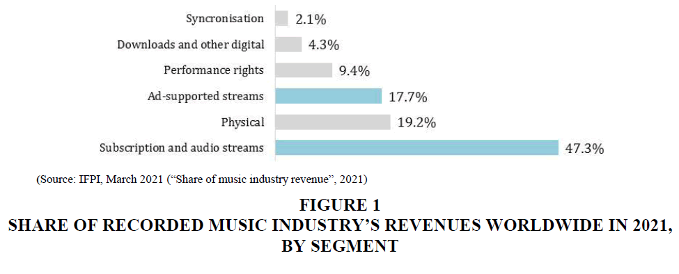
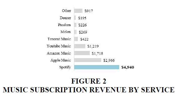
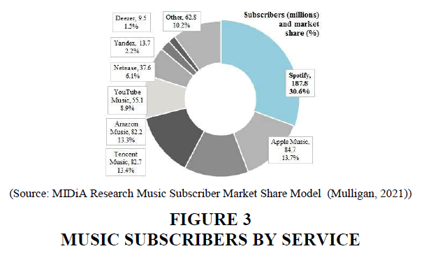
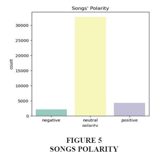
This research aims to uncover the characteristics of a popular song that could lead to sound commercial success and how well to understand and classify modern music. Try to understand this multi-faceted and highly competitive industry through its product - the 'music' by using data from the API of one of the leading music streaming platforms spotify Figures 1-5.

Literature Review

“Hit song science” was introduced by Mike McCready in the early 2000s (“Music analysis system”, 2003). It concerned the prediction of the popularity of a song using machine learning analysis of audio features and song text. However, Pachet and Roy. concluded that machine learning and related algorithms could not learn and predict the popularity of the songs using two sets of reasonable audio features (Pachet and Roy, 2008). This also validated another claim made by Dhanraj and Logan about finding a way to map hit song features (Dhanraj and Logan, 2005). Some argue that the difference in the training data amount is the issue. Today, with technological advancements and data accessibility, i intend to review this “hit song science”. Several researchers have attempted to do this in the recent past using different methodologies.

The closest to what study aims to achieve in this study is the methodology used by Khan et al. (Khan et al., 2022). They worked with a similar dataset and used feature selection algorithms to filter features based on importance and then performed some machine learning algorithms on the same to predict song popularity with convincing accuracy. Cu et al. used some very unique features to predict song popularity using Random Forrest algorithm (Cu et al., 2022) Interiano et al. also analyzed half a million top songs released in the UK between 1985 and 2015 to understand music trends and success prediction (Interiano et al., 2018)

Nijkamp, R used a purely statistical approach to establish whether each track feature influences the stream count and, in turn, the song's popularity. They created a hypothesis for each song attribute and performed regression followed by descriptive statistics analysis (Nijkamp, 2018)

Suh, Brendan Joseph also examined the effect of song attributes on the success of the music across five countries – U.S., Norway, Taiwan, Ecuador and Costa Rica - by using regression models on each song attribute (Suh, 2019). Essa et al. used regression models to predict the popularity of the songs (Essa et al., 2022), while Çimen and Kavis used statistical and regression methods to do a tie-varying analysis to quantify the effects of song features on popularity and compare them across two countries (Çimen and Kavis, 2021).

Featuring on a good Spotify playlist also is a determining factor for the success of a song on the platform. These playlists are created based on genres, and this classification of genres, as Spotify explains, does not have any fixed boundaries as the music keeps evolving and new genres form. Stern S. attempted to understand the classification of genres using music features using various supervised and unsupervised clustering algorithms (Stern, 2021). Filipcic A. explored another finding area to study how music metadata from Spotify could assist music therapy (Filipcic, 2021).

The sentiment of a song and what emotion it expresses is an essential feature in understanding the popularity of the song. I have attempted to create a new variable to factor this in. A different approach was used by a student at Warsaw University of Technology, who did sentiment analysis using text analysis on song titles and lyrics, followed by studying statistical characteristics of the melody for classification and then correlating the same with the sentiments of lyrics (“The Study of correlation”, 2020).

Methodology

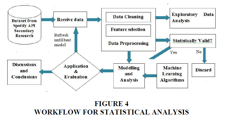
In this research, data were obtained using Spotify API using tools described later in the dedicated sub-section. This dataset was observed to be relatively clean upon preprocessing. Feature selection was performed by removing unimportant variables from the dataset. Feature generation for sentiment score was also done for this study, as described later. This was followed by Exploratory, Statistical and Predictive Data Analysis to achieve meaningful insights. Analysis was done with the established models and tests. Tools used included R- Studio for Data Collection from Spotify API, IBM SPSS for Statistical Analysis and Python in Jupyter Notebook for Predictive Analysis.

Literature Review and Hypothesis

Even though, there are large number of studies that have analyzed the impact of macro-economic variables on environment degradation but very few studies have targeted this examination towards achieving green growth. By considering this approach, we have divided the existing literature into the following broad titles and the latest studies under each section is assembled.

Data Collection

The data for this study was sourced from Spotify API, which provides developers with extensive music-related data under specific usage constraints. Using R programming and R studio, data collection was yielding a total 46, 417 records. These records encompass songs from Spotify generated playlists across various genres. The data extraction process involved specifying the market, genres, and sub-genres. For this research, the market was defined as India “list of countries”, 2015, and the genres and sub-genres were chosen based on the most streamed categories globally and within India (Naomi, 2022; Sekhose, 2019). They were as follows:

The calculation used by Spotify to determine the popularity of a song is not publicly available Table 1, although the rationale for it is - that the popularity depends on mainly two factors Tables 2 & 3.

Table 1 Genre and Subgenre
Genres	Subgenres
'pop'	'dance pop', 'post-teen pop', 'viral pop', 'indian pop'
'rap'	'hip hop', 'pop rap', 'gangster rap', 'trap'
'rock'	'album rock', 'classic rock', 'indian rock', 'hard rock'
'desi'	'filmi', 'sufi', 'modern bollywood', 'desi hip hop'
'r&b'	'urban contemporary', 'hip pop', 'new jack swing', 'neo soul'
'edm'	'electro house', 'big room', 'pop edm', 'progressive electro house'
'latin'	'tropical', 'latin pop', 'reggaeton', 'latin hip hop'
'world'	'fusion', 'gaming', 'workout','world'
'indian'	'regional', 'hindustani classical', 'punjabi', 'classical', 'devotional'

Table 2 Features of the Dataset
Track Features	‘track.id’, ‘track.name’, ‘track.artist’, ‘track.popularity’, ‘release.date’, ‘duration_ms’
Album Features	‘album.id’, ‘album.name’
Playlist Features	‘playlist.name’, ‘playlist.id’, ‘playlist.genre’, ‘playlist.subgenre’
Mood Features	‘danceability’, ‘energy’, ‘valence’, ‘tempo’
Properties	‘loudness’, ‘speechiness’, ‘instrumentalness’
Context	‘acousticness’, ‘liveness’
Segments	‘key’, ‘mode’

Table 3 Key Features Description (“Features”, no Date)
Feature	Measure	Description
Danceability	0.0 to 1.0	Interaction of specific musical elements
Acousticness	0.0 to 1.0	Probability of the track being acoustic
Energy	0.0 to 1.0	Quick, loud, and boisterous pieces
Instrumentalness	0.0 - 1.0	Vocal Free tracks will have instrumentalness 1.0
Liveness	0.0 to 1.0	Likelihood of the presence of audience during the recording
Loudness	Total volume in decibels (dB)	Typical value range is between 60 dB and 0 dB
Speechiness	Spoken words in music	Talk shows, readings from audiobooks,and poetry would be closer to 1.0
Tempo	Beats per minute (BPM)	Length of an average beat
Valence	0.0 to 1.0	Overall melodic positivity - melancholy, despondent, and angry to upbeat, joyful, and euphoric
Key	Integers mapped to pitches	Standard Pitch Class notation. E.g. 0 = C, 1 = C♯/D♭, 2 = D, No key = -1
Mode	Modality (major or minor)	Major is 1, and minor is 0
Duration	Milliseconds	Duration of track
Track Popularity	0 to 100	Based on audience interactions

Number of streams and how recent the streams are so, if the song was popular in the yesteryears but is not in recent times, then the popularity will go down. Study mainly focuses on what features make songs popular today (Alexia, 2022). On average, Spotify pays $0.003 to $0.005 to artists or rights holders of the songs per stream. That is a 30:70 split – with 30% going to Spotify and 70% to artists/rights holders. Since the number of streams determines popularity, it becomes a critical feature in studying commercial success on the streaming platform (“How much does”, no date). Also, according to the Spotify algorithm, the more a song is streamed, the more likelihood there is for the song to be further recommended by Spotify to others – so artists need to look out for that initial burst of streams to cement further popularity. Thus, Audio and technical aspects are crucial. These features must be enhanced, and significant audio components that affect the number of listens could be found if the music is to be widely listened to.

Data Preprocessing

Data cleaning is essential to improve the quality of results and improve the overall performance. Multiple steps were undertaken to clean this dataset before proceeding towards analysis. The data was obtained using the input of genre and subgenre. Thus, the Spotify algorithm pulls the tracks from playlists belonging to the genres and subgenres and adds them to create a dataset, during which several songs are repeated due to their presence in multiple playlists. At the same time, the exact genre assigned to the song is arbitrary as music is fluid, or one song could contain parts of multiple genres. Hence, i have not considered genres and subgenres as independent variables for machine-learning algorithms and thus, retaining the duplicates in dataset would be unnecessary. Thus, the duplicate tracks were removed. This reduced the number of records in the dataset from 46417 to 39147.

Columns not considered for the analysis like ‘track.artist’, ’track.album.id’, ‘track.album.name’, ‘track.album.release_date’, ‘playlist_name’, ‘playlist_id’, ‘playlist_genre’, ‘playlist_subgenre’ were removed from the dataset. Columns ‘track.name’ and ‘track.popularity’ were renamed ‘track_name’ and ‘track_popularity’. Datatypes of columns ‘track_popularity’, ‘mode’, ‘key’, and ‘duration_ms’ were converted to float. Feature generation is needed to improve performance analysis and discover compact and informative data representations. In the dataset, popularity is a target variable, and study revolves around predicting the same based on other track features. However, this ‘track.popularity’ variable is a continuous integer value ranging from 0 to 100. To utilize this as target variable, so divide it into popular and unpopular. Here consider 85% as threshold number of songs that will consider unpopular. For this, descriptive statistics of the dataset were obtained, and it was observed that the 15% mark approximately had a popularity rating of 65. Thus, all songs above the rating of 65 were considered popular, and the rest were unpopular. This gave us 5959 popular songs and 33188 unpopular songs in a dataset.

For exploratory data analysis, also divided the data into 5 popularity classes at each 20% internal. Thus, the five classes from most to least popular being ‘very high’, ‘high’, ‘medium’, ‘low’, ‘very low’. Here attempted to generate a new feature based on the sentiment expressed through the song title. To understand if the song title also has an implication on song popularity. The ‘textblob’ library was used to find the sentiment polarity in the song title (Loria, 2018). It was then classified as ‘positive’ for positive polarity, ‘negative’ for negative polarity and ‘neutral’ if polarity was ‘0.0’.

Sentiment polarity obtained using ‘textblob’ ranges from -1 to 1. This sentiment polarity for each song was then added to the data frame as a new feature.

Exploratory Data Analysis

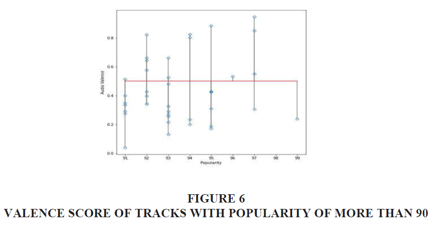
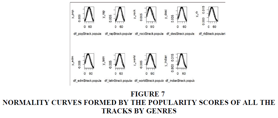
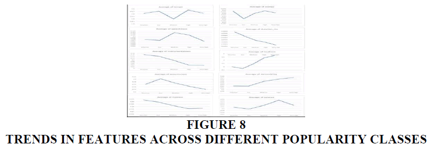
Exploratory Data Analysis is done to analyze, investigate and summarize a dataset and its main characteristics per the researcher's interpretation. For this study explored the valence scores for high popularity tracks, normal curves for each genre by popularity and the mean values of each track feature for each popularity class.

In Figure 6, The audio valence tells us about the musical positiveness about the track. The song positivity of top songs by popularity is illustrated in the above chart. The 0.5 valence line shows the threshold above which the songs are more positive (happy, cheerful, euphoric) and below which songs sound more negative (sad, angry, depressed). With around 24 tracks below 0.5 valence and 14 tracks above the 0.5 valence, the negative valence leads the chart where popularity is more than 90.

Figure 7 shows popularity of the tracks across genres shows the Normal curve. They are symmetric about the mean and show that values near the mean occur more frequently than those around others. Some genres indicate a high number of songs with zero popularity. Genres like rock, R&B, EDM, world, and Indian genres have a little asymmetry since many of their contenders have zero popularity. Meanwhile, pop, rap, Latin, and desi have more symmetry and less distribution around zero popularity. Therefore, one can say these genres can generate more popularity despite the features they possess and an artist can gain popularity in these genres more easily compared to the others.

Figure 8 shows the line charts of the mean values of the features across different popularity classes. The charts were created on excel using pivot table. The trend is significantly visible in features such as duration_ms, speechiness, instrumentalness, loudness, danceability, accousticness and liveness. Other features like tempo and valence may not show the distinctive difference, but they still show the difference between classes. The valence shows that the ‘High’ tagged popular songs are comparatively happier than the lower popularity classes, but ‘Very High’ tagged songs are less happy. The graph falls after a certain peak and the songs in ‘Medium’ and ‘High’ tag have almost the same valence.

Statistical Analysis

Statistical analysis to understand which features of a track have significant impact on the popularity of the song. Here mainly two objectives – first, to understand whether the song genre has a significant impact of song popularity. This will be done using ANOVA test as well as Post-Hoc studies and the level of significance is maintained to be 0.05. After that try to check, whether each audio feature of the track varies across the two popularity classes or not using t-independent tests Tables 4 & 5. To understand whether popularity varies across different genres Hypothesis:

Table 4 Anova Test for Popularity Across Genres
	Sum of Squares	df	Mean Square	F	Sig.
Between Groups	1379684.016	8	172460.502	332.671	0
Within Groups	20289570.8	39138	518.411
Total	21669254.82	39146

Table 5 Conclusion of Anova for Popularity Across Genres
Null Hypothesis	P-value	Conclusion
There is no significant difference in popularity across different genres	0	H0 is rejected.
		There is a significant difference in popularity across different genres.

H₀: µ₁ = µ₂ = µ₃ = µ₄ = µ₅ = µ₆ = µ₇ = µ₈ = µ₉

H₁: µ₁ ≠ µ₂ ≠ µ₃ ≠ µ₄ ≠ µ₅ ≠ µ₆ ≠ µ₇ ≠ µ₈ ≠ µ₉

H0: There is no significant difference in the popularity across different genres

H1: There is a significant difference in the popularity across different genres

The ANOVA test showed us that there is at least one pair of genres across which the popularity significantly differs. If the number of pairs is one or two, so can neglect them and consider the feature genre for popularity prediction. But if the number of pairs is high, will avoid considering the feature genre for popularity prediction.

From the exploratory data analysis and table, the number of tracks differs across genres, and variances are not homogeneous Table 6. Therefore, conducted the post hoc test of Games-Howell on the data set to understand how many pairs do not differ significantly.

Table 6 Games Howell Post-Hoc Tests
	Desi	EDM	Indian	Latin	Pop	R&B	Rap	Rock	World
Desi	-	0.941	1	0	0	0.997	0	0.701	0.113
EDM	0.941	-	0.836	0	0	1	0	0.079	0.003
Indian	1	0.836	-	0	0	0.981	0	0.796	0.152
Latin	0	0	0	-	0.78	0	0.963	0	0
Pop	0	0	0	0.78	-	0	0.143	0	0
R&B	0.997	1	0.981	0	0	-	0	0.238	0.016
Rap	0	0	0	0.963	0.143	0	-	0	0.001
Rock	0.701	0.079	0.796	0	0	0.238	0	-	0.971
World	0.113	0.003	0.152	0	0	0.016	0.001	0.971	-
Based on observed means.
The error term is Mean Square(Error) = 373.897.
*. The mean difference is significant.

To understand whether audio features vary across different popularity classes
Test: t-independent test

Hypothesis:

H₀: µ1 = µ2 = µ3 = µ4 = µ5

H₁: µ1 ≠ µ2 ≠ µ3 ≠ µ4 ≠ µ5

H₀: There is no significant difference in the features across different popularity classes

H₁: There is a significant difference in the features across different popularity classes

The following were the observations for the t-independent test for track features across popularity classes Tables 7 & 8. The popularity classes were popular and non-popular, and the level of significance was considered at 95%.

Table 7 Independent T-Test for Track Features Across Popularity Class
		Levene's Test for Equality of Variances		t-test for Equality of Means
		F	Sig.	t	df	Sig. (2-tailed)
danceability	Equal variances assumed	50.302	0	-14.079	34821	0
	Equal variances not assumed			-14.875	8087.724	0
energy	Equal variances assumed	261.046	0	-4.198	34821	0
	Equal variances not assumed			-4.777	8774.197	0
loudness	Equal variances assumed	425.732	0	-24.501	34821	0
	Equal variances not assumed			-31.536	10417.406	0
speechiness	Equal variances assumed	0.16	0.689	-0.278	34821	0.781
	Equal variances not assumed			-0.283	7799.765	0.777
acousticness	Equal variances assumed	395.058	0	11.092	34821	0
	Equal variances not assumed			12.548	8712.579	0
liveness	Equal variances assumed	67.947	0	5.908	34821	0
	Equal variances not assumed			6.486	8420.343	0
duration_ms	Equal variances assumed	349.624	0	14.239	34821	0
	Equal variances not assumed			24.507	20494.978	0
tempo	Equal variances assumed	13.682	0	-3.956	34821	0
	Equal variances not assumed			-3.879	7549.63	0
valence	Equal variances assumed	53.786	0	-10.677	34821	0
	Equal variances not assumed			-11.157	8000.574	0
instrumentalness	Equal variances assumed	2891.462	0	25.407	34821	0
	Equal variances not assumed			40.875	16811.798	0

Table 8 Conclusion of Independent T-Test for Track Features Across Popularity Class
Null Hypothesis	P-value	Conclusion
There is no significant difference in the features (except speechiness) across different popularity classes	0	H0 rejected.
		There is a significant difference in the features (except speechiness) across different popularity classes
There is no significant difference in the speechiness across different popularity classes	0.689	H0 is not rejected.
		There is no significant difference in the speechiness across different popularity classes

It was observed that each track feature was significantly varying across the popularity classes previously defined as popular and unpopular, except speechiness in this case. The difference among popularities in speechiness was significant. Therefore, further consideration was needed to study whether to use it or reject the feature. During inspection, the high popularity tracks' speechiness; with minimum 0.024 and maximum 0.685, lies between that of low popularity tracks' speechiness; minimum 0 and maximum 0.964. Since there is this distinctive difference in ranges, speechiness also has the potential to play a distinctive role in predicting whether the song will be popular or not and thus, not reject it and considered it for the ML algorithm to study its influence.

Predictive Analysis

The objective is to create a model capable of accurately predicting the popularity of a new song based on its audio features.

Data Modelling

Here, the two variables, ‘key’ and ‘mode’, were categorical, so they were converted using get_dummies function of Pandas. These dummy values were then added to data set, and the original ‘key’, ‘mode’, and ‘track_popularity’ columns were removed. The independent variables were all numeric except ‘popularity’. The dependent variable here was the binary-generated column ‘popularity’. The data was then standardized using the StandardScaler function of the sklearn’s preprocessing library. This standardization was required since the variables had different ranges to ensure uniformity during analysis and give the same relative weightage to each variable at this time. This data was then split into test and train data using the train_test_split function. The test data was kept at 20%. So there will have four sets – x_train, x_test, y_train and y_test. The training data will be used for training the machine, and the test data will be used for validation.

Logistic Regression

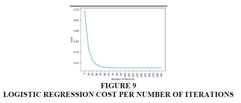
Logistic Regression is used for prediction of probability of occurrence of a binary event outcome. In this case, binary outcome is whether or not the song will be popular. Here, the logistic regression was performed. A logistic regression function was created to perform the iterative logistic regression for the best accuracy. For this function, the inputs were testing and training data for ‘input’ and ‘target’, respectively, along with learning rate and number of iterations. For testing and training data with a learning rate of 0.01 and 200 iterations, the following observation was obtained. Cross-validation scores were also obtained for the same. The average cross-validation score was 0.84733 Figures 9-12. A Grid Search CV – a cross-validation technique was also used by setting the grid and parameters to obtain the best accuracy. The best accuracy, in this case, was 0.84733 Table 9.

Table 9 Results of Logistic Regression
Accuracy	0.84733
Cross Validation Score	0.84733

KNN Algorithm

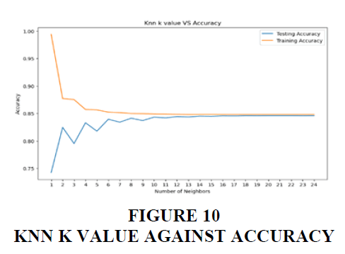
K- Nearest Neighbors is an algorithm which uses the proximity of data points as classification groups to learn and then predict using the proximity of a new data point to either of these groups Table 10. This was also done iteratively to find the best accuracy and k value. The Grid Search for Cross Validation was also performed to get the best accuracy based on setting the grid and parameters.

Table 10 Results of the KNN Algorithm
Accuracy	0.8478
Cross Validation Score	0.8482

SVM

This supervised deep learning technique can perform both regression and classification simultaneously on linear and non-linear data. The same was performed on dataset Tables 11-17.

Table 11 Results of Support Vector Machine Algorithm
Accuracy	0.84597
Cross Validation Score	0.84822

Table 12 Results of Naive Bayes Classification Algorithm
Accuracy	0.84597

Table 13 Results of Decision Tree Classifier Algorithm
Accuracy	0.7544
Cross Validation Score	0.75071

Table 14 Classification Report of Random Tree Classifier
	precision	recall	f1-score	support
0	0.85	0.99	0.91	6624
1	0.4	0.05	0.09	1206
Accuracy			0.84	7830
Macro avg	0.63	0.52	0.5	7830
Weighted avg	0.78	0.84	0.79	7830

Table 15 Confusion Matrix of Random Tree Classifier
0	6531	93
1	1144	62
	0	1

Table 16 Results of Random Forest Classifier
Accuracy	0.84163
Cross Validation Score	0.84283

Table 17 Machine Learning Performance Comparison
Model	Accuracy
LogisticRegression	0.847335
SVM	0.845977
K-NearestNeighbors	0.845977
NaiveBayes	0.845977
RandomForestClassifier	0.841635
DesicionTreeClassifier	0.754406
Lasso	0.360978
Ridge	0.354629

Naive Bayes

Naïve Bayes is a supervised learning algorithm based on the “naïve” assumption that each variable is independent and independently influences the outcome in its own capacity. The same was performed on dataset.

Decision Tree Classifier

This is a supervised learning tool that uses classification and regression to predict classes. The advantage of this is that a variable may be used at any stage of classification. Since the tree is created as a hierarchy, different variables may be considered at different hierarchical levels. Cross-validation was also performed in this case.

Random Forest Classifier

Random Forest Classifier is used to maximize prediction accuracy by averaging the accuracies of many individual decision trees. This helps to avoid issues of overfitting as well. Cross Validation was performed for this, and a confusion matrix and a classification report were generated.

Feature Importance

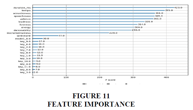
Feature Importance was done using ‘xgboost’ library and XGBClassifier function for the dataset (“XGBoost Documentation, no date”). This technique provides a score for each variable based on its usefulness or value in creating the different decision trees. It gives us a rough idea about which variables are more important for classification.

Feature importance evaluation showed that the song duration has a significant impact on the popularity of the track. The ‘duration’ track feature had an F score above 400, while key, method and sentiment had F-Score below 50 and could be potentially eliminated during analysis. For all others, the F score lay between 200 and 300.

Results

Comparison of Performance of Machine Learning Algorithms

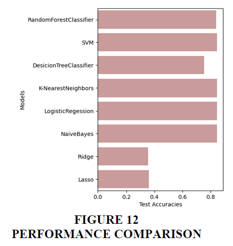
Each Machine Learning model used to predict whether the track will be amongst the top 15% showed varied accuracy levels. Now compare these to understand the scenario of the performance of models in predicting based on the individual audio attributes. Thus, Logistic Regression here has given the best accuracy of 84.7%. SVM, Naïve Bayes, KNN and Random Forest models have given similar accuracy of 84.5%. Decision Tree Classifier has given a much lesser accuracy of 75.4%.

Thus, any models amongst Logistic Regression, SVM, Naïve Bayes, KNN, Random Forest Classification could be suitable for machine learning in this case, albeit Logistic Regression had the highest accuracy. Thus, predict whether a track is popular or not based on its track features with 84% accuracy.

Discussion and Conclusion

In this research, tried to test Mike McCread’s “hit song machine” theory through exploratory data analysis and machine learning models. The Indian Market is the focus. So could understand several things about the present trends in music, which could be helpful for budding music artists to consider if they wish to follow them for higher popularity. Observed that popular songs tend to be higher in energy and loudness. At the same time, popular songs also have high instrumentalness and low speechiness. In other words, lesser words and more music is prevalent in popular songs. Popular songs were also lower in acousticness and liveness. The trendline indicating happiness emotion in a song increased until the ‘high’ popularity class and then a sharp drop was observed indicating that the most popular songs exhibit emotion of sadness. It was also observed that popular songs were shorter than non-popular ones, so the shorter the song, can say that there could be higher chance of success which have also discussed from a logical point of view. Also derived an additional feature to factor in the impact of song titles on popularity. So, a sentiment score was derived based on text analysis of the song title. This was also used in the machine learning model. Through statistical analysis and post hoc tests can concluded that genre and subgenre were not significant features to be considered for machine learning, while all other features varied significantly cross the popularity classes. Then performed several machine learning algorithms on dataset and obtained the accuracy for each, cross validation scores were also obtained and compared. On performing feature importance using xgboost, it was observed that the features – key, mode and sentiment score – do not have enough feature importance to influence the classification model. While the song duration was the attribute with the highest feature importance, all others had an f-score in the same range. Also saw that the models - Logistic Regression, SVM, Naïve Bayes, KNN, Random Forest Classification – all showed an accuracy of ~ 85%. Thus, could predict whether a song is popular or not with reasonable accuracy - corroborating Mike McCready’s “hit song machine” theory.

Further Suggestions

There are several pathways which can be further explored stemming from this reserch. Keeping the Indian Market in focus, further analysis can be done to explore the songs that machine learning models correctly predict. These song characteristics could be the most dominant as per the current data. It is also a very live topic to study as the music trend of the populous is a result of not just individual song choices but also heavily influenced by what algorithms on different platforms are recommending to them. So, a sociological approach can also be taken to understand the popularity. This could also be done through Spotify API, as Spotify also anonymously provides the listening data of individual users on its platform. Apart from this, a study can also be done over different time durations to study popular songs from different years to study the time-varying trends as music artists lean more towards favouring the algorithm. Spotify has made available the data since 2015, so a study of trends over the last nine years can be done. Apart from this, a comparative study can also be done over different target markets to understand the trends persistent in different countries. Spotify provides data for a wide array of countries, so it can also be an interesting area. Hence, as discussed previously – this is a very live study and will have to be done repeatedly to track a change in trend and also for different markets to understand the variation.

References

Alexis, M. (2022). What is the Spotify popularity index?

Çimen, A., & Kayis, E. (2021). A Longitudinal Model for Song Popularity Prediction. In DATA (pp. 96-104).

Google Scholar

Essa, Y., Usman, A., Garg, T., & Singh, M. K. (2022). Predicting the Song Popularity Using Machine Learning Algorithm. International Journal of Scientific Research & Engineering Trends, 8(2).

Google Scholar

Filipcic, A. M. L. (2021). The age of music streaming: the use of music metadata to inform music therapy clinical decisions. The Florida State University.

Indexed at, Google Scholar

Interiano, M., Kazemi, K., Wang, L., Yang, J., Yu, Z., & Komarova, N. L. (2018). Musical trends and predictability of success in contemporary songs in and out of the top charts. Royal Society open science, 5(5), 171274.

Google Scholar, Cross Ref

Khan, F., Tarimer, I., Alwageed, H. S., Karadag, B. C., Fayaz, M., Abdusalomov, A. B., & Cho, Y. I. (2022). Effect of feature selection on the accuracy of music popularity classification using machine learning algorithms. Electronics, 11(21), 3518.

Indexed at, Google Scholar, Cross Ref

Loria, S. (2018).XGBoost Documentation.

Montagu, J. (2017). How music and instruments began: A brief overview of the origin and entire development of music, from its earliest stages. Frontiers in Sociology, 2, 264256.

Indexed at, Google Scholar, Cross Ref

Mulligan, M. (2022). Music subscriber market shares Q2 2021. Midia Research, 18.

Google Scholar

Naomi. (2022). It’s here: The top songs, artists, podcasts, and listening trends of 2022.

Nijkamp, R. (2018). Prediction of product success: explaining song popularity by audio features from Spotify data (Bachelor's thesis, University of Twente).

Indexed at, Google Scholar

Pachet, F., & Roy, P. (2008). Hit Song Science Is Not Yet a Science. In ISMIR (pp. 355-360).

Google Scholar

Sekhose, M. (2019). Here’s what Indians are listening to on Spotify. The Hindustan Times.

Stern, S. (2021). Analysis of Music Genre Clustering Algorithms (Master's thesis, The University of Wisconsin-Milwaukee).

Google Scholar

Suh, B. J. (2019). International music preferences: An analysis of the determinants of song popularity on Spotify for the US, Norway, Taiwan, Ecuador, and Costa Rica.

Google Scholar

Received: 27-Dec-2024, Manuscript No. AMSJ-24-15579; Editor assigned: 28-Dec-2024, PreQC No. AMSJ-24-15579(PQ); Reviewed: 28-Jan-2025, QC No. AMSJ-24-15579; Revised: 20-Feb-2025, Manuscript No. AMSJ-24-15579(R); Published: 06- Mar-2025