Review Article: 2021 Vol: 24 Issue: 6
An inventory model with price dependent demand rates as power law form using ANT colony optimization
Satish Kumar, SRM Institute of Science and Technology
Ajay Singh Yadav, SRM Institute of Science and Technology
Veenita Sharma, Chaudhary Charan Singh University
Navin Ahlawat, SRM Institute of Science and Technology
Govindarajan Arunachalam, SRM Institute of Science and Technology
Citation Information: Kumar, S., Yadav, A. S., Sharma, V., Ahlawat, N., & Arunachalam, G. (2021). An inventory model with price dependent demand rates as power law form using ANT colony optimization. Journal of Management Information and Decision Sciences, 24(6), 1-10.
Abstract
The main object of keeping inventories is to meet market demands using Ant Colony Optimization for Traveling Salesman Problem. Typically, retailers face a wide range of demands for different types of goods. These demands are not under the control of the organization using Ant Colony Optimization for Traveling Salesman Problem. In the present paper, demand taken as price dependent as power law form as well as time. The rate of deterioration and holding cost are considered also time dependent using Ant Colony Optimization for Traveling Salesman Problem. Shortages are allowed with partial backlogged using Ant Colony Optimization for Traveling Salesman Problem. Results are illustrated along with sensitivity analysis.
Keywords
Inventory; Price dependent demand rates; Ant colony optimization; Traveling salesman problem.
Introduction
Normally every businessman, maintain stock of goods for smooth running of business operation. The EOQ models are most successful models because they are very simple to understand and apply. But the situation of demand is different in today market where demand is always varies with time and selling price etc. So, in the present inventory model, the authors decided to take variable demands rate i.e. time and price dependent demand rate, which better match with real market situations.
There are many inventory models already developed under the considering time dependent demand rate. Demand of any product uniformly change in linear time-dependence demand rate, which is not always, happens in the actual market for any product. However, demand rate in quadratic time-dependence is seems better compare with linear. Finally, there is extraordinarily high change in demand due to exponential rate which can’t see in real market. The time dependent demand rate oriented researches are very restrictive. Silver and Meal (1969) first introduced an inventory model for time varying demand pattern. After that, there are many contributions came from researchers in this direction. Lin et al. (2000); Goyal and Giri (2003); Singh and Pattnayak (2014) presented a model for two warehouses with linear rate of demand. Sicilia (2015) presented an inventory system with power law rate of demand and uniform replenishment. Tripathi et al. (2017); and Xu et al. (2018) present a model considering the demand rate as stock dependent. Recently, Wang et al. (2019) gives a model taking time dependent demand rate under trade credit and inflation. Now, we know that cost of any item is an important part to decide the item demand. In general, product with higher price has less demandable and converse. For defective goods, this argument is more applicable whose demand is always price dependent. Therefore, price decisions are useful as well as essential. Whitin (1955) first introduced a model taking price dependent demand depend rate. Heydari and Norouzinasab (2015) presented a model considering demand as price-sensitive. The authors feel that the demand of items much better represented by time and selling price of item. So, in present model, we are taken the demand rate as inversely proportional to price. When item will be out of stock the demand will be dependent on only price. The conditions like deterioration, variable holding cost and partial backlogging also considered. Minimization cost technique considered. Supply chain management can be defined as: "Supply chain management is the coordination of production, stock, location and transportation between actors in supply chain to achieve the best combination of responsiveness and efficiency to a given market. Many researchers in the inventory system have focused on products that do not exceed deterioration. However, there are a number of things whose significance does not remain the same over time. The deterioration of these substances plays an important role and cannot be stored for long (Yadav et al., 2020a,b,c). Deterioration of an object can be described as deterioration, evaporation, obsolescence and loss of use or limit of an object, resulting in lower stock consumption compared to natural conditions. When commodities are placed in stock as inventory to meet future needs, there may be deterioration of items in the system of arithmetic that may occur for one or more reasons, etc. Storage conditions, weather or humidity (Yadav et al., 2019a,b). Inach it is generally claimed that management owns a warehouse to store purchased inventory. However, management can, for a variety of reasons, buy or give more than it can store in its warehouse and name it OW, with an additional number in a rented warehouse called RW located near OW or slightly away from it (Yadav et al., 2016; 2017a,b). Inventory costs (including holding costs and depreciation costs) in RW are usually higher than OW costs due to additional costs of handling, equipment maintenance, etc. To reduce the cost of inventory will economically use RW products as soon as possible. Actual customer service is provided only by OW, and in order to reduce costs, RW stocks are first cleaned. Such arithmetic examples are called two arithmetic examples in the warehouse (Yadav and swami, 2018a,b; 2019a,b). Impact of liquidity and management efficiency on profitability: An empirical study of selected power distribution utilities in India (Azhar, 2015). Impact of financial leverage on market value added: empirical evidence from India (Pandya, 2016). Inference of FDI in Indian retail sector: Some Reflections (Deshpande et al., 2014). Job Satisfaction in IT Department of Mellat Bank: Does Employer Brand Matter? (Tajpour et al., 2021). Studying the influence of emotional intelligence on the organizational innovation (Tajpour et al., 2018).
Assumptions and Notations
Assumptions and notations for present model-
1.  = the purchase cost/unit taken as constant of the item.
2. ‘K’= the cost of order per cycle.
3. Lead time is zero.
4. 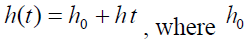 is the initial holding cost and
5. ‘p’= the selling price for every unit item.
6. 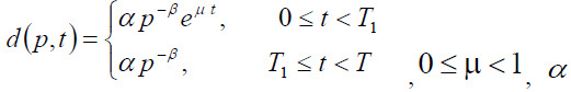 be the scale and β be the shape parameter of demand curves.
7.  is the decay rate.
8. ‘T’ is the cycle length.
9. QT be the highest stock level.
10. Shortages with backlogged rate are permitted defined by 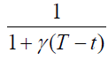 where
where .
.
11. T1 Shortage starting time.
12. ‘s’ shortage cost/unit/year.
13. 'π ' per unit opportunity cost for lost sales.
The Model and Solution
In this section, a perishable item replenishment policy with partial backlog is considered. The Figure 1 shows the behavior of the inventory system.

Figure 1 The Behavior of the Inventory System
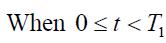
Let I(t) be the level of inventory at any time t. The change in inventory w.r.to t defined as
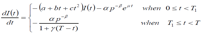 (1)
(1)
Under condition, I(T1) = 0 (2)
Now, from (1),

 (3)
(3)
And
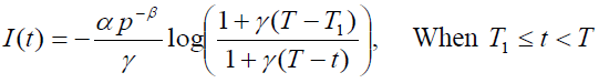 (4)
(4)
Where I(0) is consider as initial stock. Ignoring the power more than one of a, b, c and μ . Taking Z(t) be the stock which are loss due to deterioration of items during the interval [0, t].
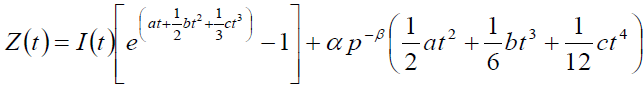 (5)
(5)
Using equation (2) in equation (5), we have
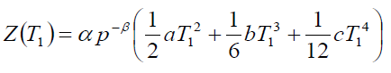 (6)
(6)
Also the total demand in the interval
 (7)
(7)
Therefore, ordered quantity per cycle is
QT = Total decay + Total demand in the interval [0, T1]
 (8)
(8)
Since 
Therefore, from equation (3), we can

 (9)
(9)
Therefore
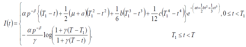 (10)
(10)
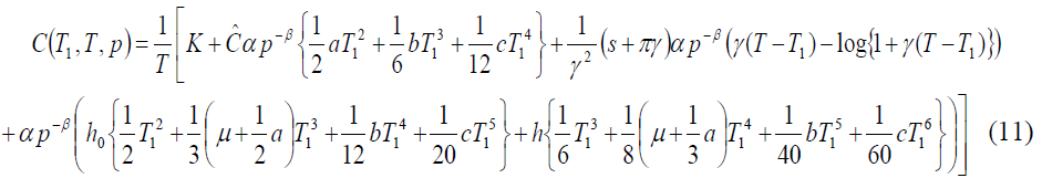
The average system cost is given by
Also, the order rate is
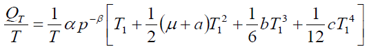 (12)
(12)
Now, the behavior of the order rate w.r.to a, b, c and μ is determined by
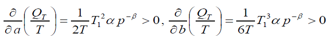
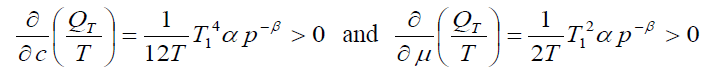
Also with respect to price ‘p’ is
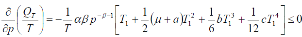 (13)
(13)
Thus, the order rate increase if increases in a, b, c and μ and decrease with increase in p. Now, our objective is to obtain values of T1, T and p which make C(T1, T,p) as minimum. The necessary condition for C(T1, T,p) as minimum are
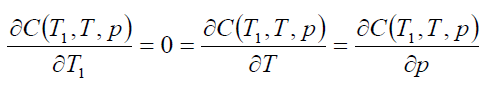

 (15)
(15)

 (16)
(16)
Solving (14), (15) and (16) simultaneously and find T1, T & p for which function C(T1, T,p) will be minimum.
Working of ACO for TSP
Initially, each ant is placed at random on a city. When developing a viable solution, the ants select the next city to visit using a probabilistic decision rule. When an ant k declares in city i and constructs the partial solution, the probability of moving to the next neighboring city j i is given by
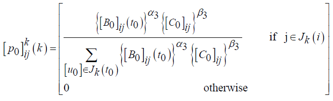 (17)
(17)
Where  is the intensity of trails between edge (i,j) and
 is the heuristic visibility of
the edge (i, j), and
is the heuristic visibility of
the edge (i, j), and 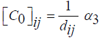 Is the influencing factor of pheromones,β3 is the influence of the
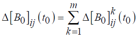
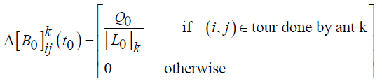
local node, and Jk (i) is a set of cities that remain to be visited when the ant is in city i. Once each ant
has completed their turn, the amount of pheromones on each path will be adjusted with the following
equation.
Is the influencing factor of pheromones,β3 is the influence of the
local node, and Jk (i) is a set of cities that remain to be visited when the ant is in city i. Once each ant
has completed their turn, the amount of pheromones on each path will be adjusted with the following
equation.
 (13)
(13)
is pheromone evaporation coefficient and ρ where
 (14)
(14)
 (18)
(18)
(1-ρ ) is the decay parameter of pheromones (0<ρ<1) where it represents the evaporation of the track when the ant chooses a city and decides to move. Lk is the length of the turn for each formed per ant k and m is the number of ants. Q is the pheromone deposition factor.
Case Study
In this section, we consider numerical examples with data same as reference research with appreciate units to illustrate the models numerically.

Then the optimal result of the model is

Sensitivity Study
The aim of present section is to identify parameters to the changes of which the solution of the model is sensitive.
| Table 1 Sensitivity Study α | |||||
| Parameter Value | % Change | T | T1 | QT | C |
| 80000 | -20 | 1.08385 | 0.44729 | 62.65580 | 367.87000 |
| 90000 | -10 | 1.02208 | 0.42422 | 66.76390 | 390.11200 |
| 110000 | +10 | 0.92488 | 0.38734 | 74.73440 | 431.14800 |
| 120000 | +20 | 0.88567 | 0.37226 | 77.88210 | 450.25900 |
| Table 2 Sensitivity Study for β | |||||
| Parameter Value | % Change | T | T1 | QT | C |
| 1.20 | -20 | 0.51416 | 0.22352 | 138.22600 | 776.26300 |
| 1.35 | -10 | 0.70617 | 0.30173 | 99.09240 | 564.89400 |
| 1.65 | +10 | 1.33248 | 0.53726 | 50.00220 | 299.26400 |
| 1.80 | +20 | 1.83340 | 0.70511 | 35.04770 | 217.78700 |
| Table 3 Sensitivity Study For μ | |||||
| Parameter Value | % Change | T | T1 | QT | C |
| 0.08 | -20 | 0.97146 | 0.40670 | 70.76290 | 410.74800 |
| 0.09 | -10 | 0.97064 | 0.40559 | 70.70650 | 410.94700 |
| 0.11 | +10 | 0.96903 | 0.40340 | 70.59550 | 411.34100 |
| 0.12 | +20 | 0.96824 | 0.40233 | 70.54100 | 411.53600 |
Observations
From above Tables 1,2 & 3, we observed that:
• It is observed that duration of the cycle length have negative correlation corresponding to the parameters α and μ but have positive correlation corresponding to the parameters β Also, model is more sensitive for the parameters β comprising to other parameters
• The average cost of the system has negative correlation with respect to the parameter β but have positive correlation w.r.to α and μ.Also it is noted that the model is more sensitive for the parameters β comprising to other parameters.
• From the above points, we can say that sufficient care should be about parameter β in conducting model.
Conclusions
This model developed under considering the demand rate as time and price during available inventory and price dependent during shortages with backlog rate depend on waiting time using Ant Colony Optimization for Traveling Salesman Problem. Demand function have negative derivative with respect to price i.e. demand is a decreasing when selling price of items is increasing using Ant Colony Optimization for Traveling Salesman Problem. Variable holding cost is taken in account. To find approximate results cost minimization technique is applied using Ant Colony Optimization for Traveling Salesman Problem. The problems are illustrated numerically. In, future studies the present model will be more realistic after considering such as stock dependent demand rate, life time items, trade credit policy, lead time, Weibull distribution and considering inflation etc.
References
- Azhar, S. (2015). Impact of liquidity and management efficiency on profitability: An empirical study of selected power distribution utilities in India. Journal of Entrepreneurship, Business and Economics, 3(1), 31-49.
- Deshpande, M., Gaddi, A., & Patil, S. R. (2014). Inference of FDI in Indian retail sector: Some Reflections. Journal of Entrepreneurship, Business and Economics, 2(2), 82-97.
- Goyal, S. K. & Giri, B. C. (2003). The production-inventory problem of a product with time varying demand, production and deterioration rates. European Journal of Operational Research, 147, 549-557.
- Heydari, J., & Norouzinasab, Y. (2015). A two-level discount model for coordinating a decentralized supply chain considering stochastic price-sensitive demand. Journal of Industrial Engineering International, 11, 531-542.
- Lin, C., Tan, B., & Lee, W. C. (2000). An EOQ model for deteriorating items with time-varying demand and shortages. International Journal of System Science, 31(3), 391-400.
- Pandya, B. (2016). Impact of financial leverage on market value added: empirical evidence from India. Journal of Entrepreneurship, Business and Economics, 4(2), 40-58.
- Sicilia, J., González-De-la-Rosa, M., Febles-Acosta, J., & Alcaide-López-de-Pablo, D. (2015). Optimal inventory policies for uniform replenishment systems with time-dependent demand. International Journal of Production Research, 53(12), 3603-3622.
- Silver, E. A., & Meal, H. C. (1969). A simple modification of the EOQ for the case of the time varying demand rate. Production of Inventory Management, 28, 52-65.
- Singh, T., & Pattnayak, H. (2014). A two-warehouse inventory model for deteriorating items with linear demand under conditionally permissible delay in payment. International Journal of Management Science and Engineering Management, 9, 104-113.
- Tajpour, M., Moradi, F., & Jalali, S. E. (2018). Studying the influence of emotional intelligence on the organizational innovation. International Journal of Human Capital in Urban Management, 3(1), 45-52.
- Tajpour, M., Salamzadeh, A., & Hosseini, E. (2021). Job Satisfaction in IT Department of Mellat Bank: Does Employer Brand Matter? IPSI BgD Transactions on Internet Research, 17(1), 15-21
- Tripathi, R. P., Pareek, S., & Kaur, M. (2017). Inventory models with power demand and inventory-induced demand with holding cost functions. American Journal of Applied Sciences, 14(6), 607-613.
- Wang, L., Chen, Z., Chen, M., & Zhang, R. (2019). Inventory policy for a deteriorating item with time-varying demand under trade credit and inflation. Journal of Systems Science and Information, 7, 115-133.
- Whitin, T. M. (1955). Inventory control and price theory. Management Science 2, 61-68.
- Xu, C., Zhao, D., & Min, J. (2018). Optimal inventory models for deteriorating items with stock dependent demand under carbon emissions reduction. Systems Engineering - Theory & Practice. 38, 1512-1524.
- Yadav, A. S., & Swami, A. (2018a). A partial backlogging production-inventory lot-size model with time-varying holding cost and weibull deterioration. International Journal Procurement Management, 11(5), 639-649.
- Yadav, A. S., & Swami, A. (2018b). Integrated Supply Chain Model for Deteriorating Items With Linear Stock Dependent Demand Under Imprecise And Inflationary Environment. International Journal Procurement Management, 11(6), 684-704.
- Yadav, A. S., & Swami, A. (2019a). A Volume Flexible Two-Warehouse Model with Fluctuating Demand and Holding Cost under Inflation. International Journal Procurement Management, 12(4), 441-456.
- Yadav, A. S., & Swami, A. (2019b). An inventory model for non-instantaneous deteriorating items with variable holding cost under two-storage. International Journal Procurement Management, 12(6), 690-710.
- Yadav, A. S., Abid, M., Bansal, S., Tyagi, S. L., & Kumar, T. (2020a). FIFO & LIFO in Green Supply Chain Inventory Model of Hazardous Substance Components Industry with Storage Using Simulated Annealing. Advances in Mathematics: Scientific Journal, 9 (7, 5127-5132.
- Yadav, A. S., Bansal, K. K., Kumar, J., & Kumar, S. (2019a). Supply Chain Inventory Model For Deteriorating Item With Warehouse & Distribution Centres Under Inflation. International Journal of Engineering and Advanced Technology, 8(2S2), 7-13.
- Yadav, A. S., Bansal, K. K., Shivani, Agarwal, S., & Vanaja, R. (2020b). FIFO in Green Supply Chain Inventory Model of Electrical Components Industry With Distribution Centres Using Particle Swarm Optimization. Advances in Mathematics: Scientific Journal. 9(7), 5115-5120.
- Yadav, A. S., Kumar, J., Malik, M., & Pandey, T. (2019b). Supply Chain of Chemical Industry For Warehouse With Distribution Centres Using Artificial Bee Colony Algorithm. International Journal of Engineering and Advanced Technology, 8(2S2), 14-19.
- Yadav, A. S., Mishra, R., Kumar, S., & Yadav, S. (2016). Multi Objective Optimization for Electronic Component Inventory Model & Deteriorating Items with Two-warehouse using Genetic Algorithm. International Journal of Control Theory and applications, 9(2), 881-892.
- Yadav, A. S., Sharma, N., Ahlawat, N., & Swami, A. (2020c). Reliability Consideration costing method for LIFO Inventory model with chemical industry warehouse. International Journal of Advanced Trends in Computer Science and Engineering, 9(1), 403-408.
- Yadav, A.S., R. P. Mahapatra, Sharma, S., & Swami, A. (2017a). An Inflationary Inventory Model for Deteriorating items under Two Storage Systems. International Journal of Economic Research, 14(9), 29-40.
- Yadav, A.S., Taygi, B., Sharma, S., & Swami, A. (2017b). Effect of inflation on a two-warehouse inventory model for deteriorating items with time varying demand and shortages. International Journal Procurement Management, 10(6), 761-775.