Keywords

BSM, Taguchi Method, ANOM, S/N Ratio, ANOVA, Tukey Method.

Introduction

The Design of experiment using the Taguchi orthogonal array approach can economically satisfy the needs of solving problem and products design optimization projects. By applying the Taguchi’s method researchers, engineers and scientists can reduce the time, resources and money required for little experimental investigation. The DOE gives the relation between the input and output variables. The DOE using the Taguchi Orthogonal array approach requires a good planning, wise arrangement of the experiments and analysis expert of results. The Taguchi’s method became the standard method for DOE application. It was developed by Dr Genechi Taguchi (a Japanese engineer, 1940). It became one of the best DOE for scientists and engineers.

The main aim of the DOE is to get more and realistic information regarding the input and output variables. In order to get the more and realistic information, a large number of experiments are required but the modern theory of experiments proves that it is not always true. The maximum number of experiments, the huge will be error and it led to more costly. It is better to gather the more and realistic information while doing the fewer experiments. One of the best and better examples is Taguchi’s method. The Taguchi has developed a method in order to study the whole process parameters with only minimum balanced trials, called orthogonal array. The main aim of DOE (Taguchi’s method) is to look which parameter (input) effects more on output. It is a well-known, powerful and unique approach to product quality improvement.

There are two main approaches to DOE, Full Factorial design (FFD) and the Taguchi’s method. FFD is a set of an experiment whose design consists of more than one factors each with discrete possible level and whose experiment units takes all possible combinations of all those levels across all such factors. For example, if there are K factors each at 3 levels, FFD has 4^K runs. This for 4 factors at 3 levels it would take 81 trials runs. The Taguchi method is a statistical tool developed by Genier Taguchi (1940) a Japanese engineer, proposed a model for experiment design. The Taguchi experiment array design is using to arrange the parameters affecting the process and the levels of which they should be varied. Instead of having all possible experiment like FFD, Taguchi model provides a minimum number of experiments. In case of 4 factors and 3 levels, it would take 9 trials runs. The experiments are not randomly generated but they are based on judgmental sampling. It reduces time, resources and cost.

In this paper, the Taguchi method is using in order to do an experiment on BSM for European call option (BSM-ECO) at one period. The paper looks at the effects of four parameters in the BSM-ECO at one period, the underlying asset price, the strike price, interest rate and the volatility. The Taguchi’s orthogonal array L9 (3^4) is used in order to estimate the factors that influence the performance criteria and also which factors are more important than others. The Analysis of Mean (ANOM), S/N ratio, Tukey Method and Analysis of variance (ANOVA) is used in order to get the objectives of this paper. In order to develop a DOE by using Taguchi method. The following points are necessary:

1. Define the response variable, in this study the response variable is the value of the European call option.

2. Select the input variables, there are four input variables that are: Underlying asset, strike price, interest rate and volatility in order to estimate the value of call option.

3. Select the number of levels, in this study we choose three levels as shown in Table 1.

Table 1 Data for Calculating the Call Option Value by Using Bsm-Eco
Levels↓	Parameters →	S0	K	r	σ
1		130	100	5%	20%
2		140	105	6%	21%
3		150	110	7%	22%

4. Select the orthogonal array, it is based on the 2^nd and 3^rd point. In this study we want to conduct an experiment in order to understand the influence of four independent with each having three set values on a call option, then L9 orthogonal array might be the right choice. It allows us to consider a selected subset of combinations of multiple factors at multiple levels.

5. Assigning the four independent variables to each column

6. Conduct the experiment

7. Analysis the data (the call option)

Therefore, it is necessary for an option holder to know which parameter effects more and how much it effects on the call option. In order to know about it, the ANOM describes the best combinations of the parameters where the value of European call option is more and also it identify which parameter affects more on the put option. The ANOVA used in order to measure the percentage contribution of each independent on the put option.

Literature Review

Now a day’s Taguchi’s method is using in every field such as producing planning, education, service system, Software testing (Lazic), Environmental Engineering, Biotechnology. The Taguchi’s method is a methodical approach for expansion of various factors with considering to performance, cost and quality (Phadke, 1989). It offers the standard quality of a product is estimated by standard characterizes such as; larger is better, nominal is the best, smaller is better (Roy, 2001; Phadke, 1998).

Fang and Wang (2002), used some factors or inputs such as material, depth of cut, feed rate cutting tool point angle, cutting time and spindle speed in order to develop a real model for the measuring the surface roughness in finish turning.

Silva et al. (2014) used the Taguchi’s method to environmental engineering in order to evaluate advanced oxidative processes in Polyester-Resin waste water treatment. It shows that the Taguchi’s method is a useful tool for environmental engineering.

Thomas (2008) solved a class optimization engineering problems experienced in systems engineering and architecting by using the Taguchi orthogonal approach.

Athreya & Venkatesh (2012) illustrated the procedure adopted in using Taguchi method to a lathe facing operation. In this study, they compare both the FFD and Taguchi’s method and got the similar result.

Chan et al. (2014) investigated the factors of four reaction parameters, a) type of catalyst, b) reaction temperature, c) catalyst loading and d) nitrogen gas flow-rate on a liquid yield from the catalytic pyrolysis of EFB (Empty Fruit Bunch). This investigation was based on the Taguchi’s L9 (3^4) orthogonal array. The catalyst loading has the most effective factor on the basis of signal-to-noise (S/N) ratio using higher the better criteria.

Shravani et al. (2011) used the Taguchi’s L9 orthogonal array design in order to prepare and optimise the various parameters of enteric coated pellets. By using the L9 orthogonal array it reduces the time and also provides idea formulation.

Rao and Padmanabhan (2012) used the Taguchi’s L9 orthogonal array design that how parameters (voltage, electrolyte and feed rate) concentration on MRR (metal removal rate). The ANOVA, Regression analysis and S/N ratio have been used in order to analyse the effects of these parameters. The feed rate affects more on MMR.

Dar and Anuradha (2018) used Taguchi orthogonal L9 array, ANOM and ANOVA in order to identify which parameter affects more on the probability of default. It was identified that the volatility affects more on the probability of default. (Kacker et al., 1991, Lee et al., 2003, Lee et al., 2003, Yang & Tarng 1998, Shangi 2002).

The aim of the experimental is to get the maximum realistic information. A large number of variables demand a large number of measurements to get maximum realistic information. The modern theory of experiments proves that it is not always true that higher number of measurements will give maximum realistic information. Larger the number of measurements, huge will be the total error that enters into the measurement equation. A Larger number of measurements led to more costly experimentation. It is necessary to obtain the maximum information while doing a minimum number of experiments. One of the best examples is the Taguchi method. The DOE program is to look which factor effects more on the output of an experiment.

Objectives

As per literary review, we found that the researchers have so far worked on option pricing model using Taguchi’s orthogonal array design whereas Taguchi’s model can be used in option pricing also. The objectives of this study are:

• To identify the best level for each parameter.

• To measures which factors are more important than others.

• To check whether the value of a call option follows a certain distribution.

• To measure the percentage contribution of each parameter.

Methodology

The aim of this paper is to do an experiment on the BSM-ECO at one period at three levels. The Taguchi’s method (L9 (3^4)) is used to run the trials. In Taguchi’s method, only 9 experiments are used instead of 81 as per FFD. The date is taken from the published paper (Dar and Anuradha 2017) because it gives the complete information to measure the value of the call option by using BSM given in Table 1. Finally, the ANOM, S/N ratio, Tukey method is used to look which factor affects more or less and ANOVA gives the percentage contribution of the variables.

European Call Option

“It is a contract that gives rights to owner, but not obligation to buy the underlying asset ( S₀) at a specified price (strike price K) within a specified time (T). It will not exercise before the maturity date. The buyer of the call option believes that the price of an underlying asset S_T goes up in a future date. In this case, the buyer of the call option will decide whether to exercise or not because he is havings the rights. At the expiry date T, if the price of the underlying asset S_T is less than strike price . Then the call option is not exercised and if the price of an underlying asset at maturity time is greater than the strike price, then he will exercise it, i.e., the holder buys the underlying asset from the strike price K and sells it to the market”. The Black and Scholes developed a formula in order to estimate the values of European call and put option in 1973 (Black and Scholes 1974, Merton 1974, Dar and Anuradha 2017, Hull 2016).

The Black-Scholes formula for European call option without dividend paying is:

Where N(*) is the standard cumulative distribution function

“ S_t is the price of an underlying asset at time t , K is the strike price, r is the risk free rate of the interest, (T-t ) is the mature time, σ is the volatility of the return of the underlying asset, N(* ) cumulative distribution function of the standard normal distribution”.

Note: a) The European style means that the contract will expire only at a set date or maturity date. b) In case of call option the underlying asset at mature date must be greater than K.c) S_t * N(d₁) is the present value of the underlying asset if the option is exercised and d) K * e^-r(T-t) is the present value of the strike price K if the option is exercised.

Design of Experiment (Doe) Using Taguchi Orthogonal Array

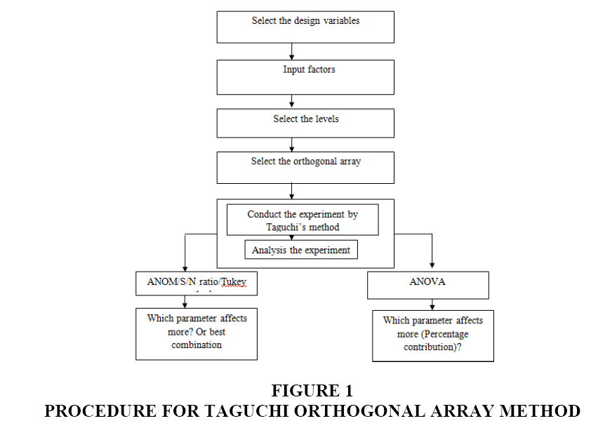
Taguchi method is a popular statistical model developed by G. Taguchi. At starting it was used for only improving the quality of products (mainly manufactured goods). Nowadays it is used in every field in order to minimise the number of trials, time, cost and resources. This method is based on the orthogonal array experiments which give a much-reduced variance for the experiment with the optimum setting. Taguchi orthogonal array design is a type of design that is based on a design matrix and it allows you to consider a selected subset of combinations of various factors at different levels. It is the balanced and ensures that all levels of all parameters are considered equally. In this study, the four parameters are varied at three levels and on the bases of levels and parameters, the orthogonal array L9 is selected (Figure 1).

The experiment runs with four parameters at three levels are determined by using the Taguchi L27 orthogonal array. The MINITAB software determines 9 trails instead of 81 as per FFD. The four parameters in this study are: Underlying asset S₀, strike price , interest rate r and volatility σ at three levels are summarised in Table 1.

In this study, we are working on the European call option using BSM, the parameters S₀, K, r and σ are used as input parameters. Table 2 shows all combinations that are required according to Taguchi’s model and the parameter value of call option using the equation (1). The experiment layouts for put option process parameters by using Taguchi L9 approach shown in Table 2. These experiments are not randomly selected but it is based on some well-defined procedure or sampling. The Taguchi L9 orthogonal array approach is appropriated for experimentation and the experimental matrix along with result (value of European call option) using equation (1) is shown in Table 2.

Table 2 Taguchi’s L9 (3^4) Orthogonal Array for European Call Option Using Bsm
Experiment	S0	K	r	σ	Call option value
1	130	100	0.05	0.20	35.44027
2	130	105	0.06	0.21	32.18835
3	130	110	0.07	0.22	29.25158
4	140	100	0.06	0.22	46.18057
5	140	105	0.07	0.20	42.44147
6	140	110	0.05	0.21	36.32111
7	150	100	0.07	0.21	56.86112
8	150	105	0.05	0.22	50.45923
9	150	110	0.06	0.20	46.71759

Result, Analysis and Discussion

Model Summary

Table 3 R-sq is a regression coefficient. It is a statistical tool that measures how much the data is close in order to fit the regression line. In this model R-sq value is 99.98% which indicates that the fit of the experimental data is satisfactory. The R-sq is approximately equal to 1 that means the regression line perfectly fits the data. S is the standard deviation of the data points. It indicates that how far a data fall from the fitted value. Less standard deviation means better the model describes the response.

Table 3 Model Summary
S	R-sq	R-sq (adj)	R-sq (pred)
0.159971	99.98%	99.97%	99.88%

The Minitab software was used in order to model for the call option value, the regression equation is given below:

Regression Equation

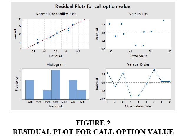
The following points explain the Figure 2.

a. In normal probability plot, there is no outliers exist which means that the values of call options (data) follow a normal distribution and the factors are influencing the response.

b. In versus fits plot (fitted value vs. residual), the plot indicates that the relationship between the data is non-linear and the variance is constant.

c. The Histogram indicates that there is no outlier exists and the data are not skewed.

d. In versus plot (residuals versus observation order), the plot indicates that the data have systematic effects.

ANOM

The response mean (ANOM) is the average response for each combination of control parameters (factors) levels in a statistic Taguchi method. The aim of this method is to identify which parameter effects more on put option and also it determines the best combination where the European call option gets maximum value. For each parameter, Minitab software measured the average of the response (call option value) at each level of the parameter. The delta identifies the size of effect by the taking the difference between the highest and the lowest value of average for a parameter and the rank in the response Table 4 helps us to identify which parameter effects more. The parameter with the highest delta value is given rank 1, the parameter with the second highest delta is given rank 2 and so on.

Table 4 Response Table for Mean (Anom)
Level	S0	K	r	σ
1	32.2934	46.16065	40.7402	41.53311
2	41.64772	41.69635	41.6955	41.79019
3	51.34598	37.43009	42.85139	41.96379
Range	19.05258	8.73056	2.111187	0.430683
Rank	1	2	3	4

The selected numbers (bold) in Table 4 are the maximum in every column, as per range we set the ranking for all the parameters (higher range=rank 1 and so on). We conclude that the best combination is S₀3 * K1 * r3 * σ3.

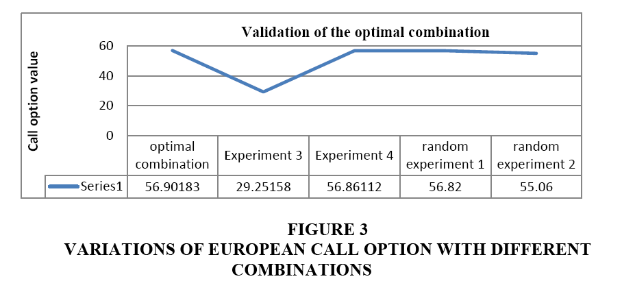
The best combination has been determined S₀3 * K1 * r3 * σ3 because it will provide us maximum value of call option. In order to prove, we will choose some combinations from the given table (Experiment No. 3 and 4) and some random combinations are selected. The variations of call options with different combinations are presented in Figure 3. It is shown that the optimal combination has the highest value (56.90183) than all four combinations and also we assume that there exist the additively of effects of different parameters (Wang et al., 2016).

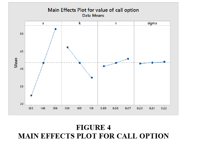
The ANOM gives us an idea about which parameter affect more on option pricing using BSM. The rank indicates that the underlying asset S₀ affects more and the volatility σ affects less on call option using BSM.

Figure 4 indicates that how the parameters affect the call option value using BSM. It clearly shows that underlying S₀ or S asset effect more as compared to others and the sigma effects less.

Signal-to-Noise Ratio (Larger-is-Best)

The experiment layout using Taguchi L9 orthogonal array with responses values of European call option using BSM. The S/N ratios of all the four parameters at three levels were calculated and are shown in Table 5.

Table 5 Response Table for Signal to Noise Ratios Larger is Better
Level	S0	K	r	σ
1	30.16	33.13	32.08	32.31
s2	32.35	32.26	32.28	32.15
3	34.18	31.31	32.33	32.22
Delta	4.03	1.82	0.24	0.16
Rank	1	2	3	4

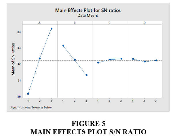
The underlying asset price S₀ (Delta=4.03, Rank=1) has the largest effect and volatility (Delta=0.16, Rank=4) has the smallest effect on call option. As per Table 5 the rank indicates that which factor effects more on the European call option using BSM.

In order to measure which factor effects more on response variables? The best method is to compare the slope of lines with relative magnitude.

If the line in Figure 5 is horizontal then there is no effect. But all the lines are not horizontally which mean that each factor effects on the call option. It clearly shows that underlying asset S₀ or S(A) effect more as compared to others and the volatility (D) effects less.

We can use Tukey method also in order to identify which parameter effects more in call option using BSM.

Tukey Pairwise Comparisons

In this result, the Table 6 shows that the group A contains factor S₀, B contains factor K and C contains σ and r. The result shows that it is not sharing any letter. The groups that shares the letter are not significant different. Factor S₀ and K is not sharing the letter, which indicates that has a significantly higher mean than factor , σ and r.

Table 6 Grouping Information Using the Tukey Method and 95% Confidence
Factor	N	Mean	Grouping
S0	9	140.00	A
K	9	105.00		B
r	9	0.21000			C
σ	9	0.06000			C
Note: Means that do not share a letter are significantly different

ANOVA

In order to measure the percentage contributions of each independent variable in European call option using BSM. An application of ANOVA is used in order to estimate the percentage of each parameter. It shows the relation between the response variable and the predictor variable. In order to estimate the percentage contribution, we need regression model known as ANOVA. It is defined as “sum of squares of a parameter by total sum of squares”. Table 7 shows the contribution of each parameter.

Table 7 Percentage Contribution
Source	Adj SS	Adj MS	F-Value	P-Value	Percentage contribution	Rank
S	544.501	544.501	21277.24	0.000	81.77%	1
K	114.334	114.334	4467.78	0.000	17.17%	2
r	6.686	6.686	261.25	0.000	1.004%	3
σ	0.278	0.278	10.87	0.030	0.0424%	4
Error	0.102	0.026
Total	665.901
Note: At 95% confidence interval (α = 0.05)

The percentage contribution of the parameters that are shown in Table 7 can be calculated as:

The P-value of all the parameters are less than (α = 0.05 ), because of this we can conclude that there is a statistically significant differ. So, all the factors are effects on call option differently. In order to measure which parameter effects more or less on call option at one period, the ANOVA is used.

The percentage of each parameter is defined as the significance rate of the process parameters on the value of call option. The percentage (%) numbers represent that the underlying asset price at time t=0, the strike price, the interest rate and the volatility have a significant effect on pricing of European call option using BSM. It can be observed in Table 8 that the underlying asset price at time (t = 0 ) S₀, the strike price , the interest rate r and volatility σ effects the call option by 81.77%, 17.17%, 1.004% and 0.0424% respectively.

Conclusion

This study discussed an application of the Taguchi L9 orthogonal array. It is based on the European call option using BSM at one period. The four parameters: The underlying asset , the strike price K, the interest rate r and the volatility σ on European call option at three levels are used. The conclusion of this study is summarised below:

a. The values of a call option follow a normal distribution because the values approximately in a straight line and there are no outlier exist.

b. The ANOM is being used in order to identify the best level for every four parameters. The best combination in this study is S₀3 * K1 * r3 * σ3.

c. The ANOM and S/N ratio is being used in order to explain which parameter effects more or less on European call option using BSM. The Rank that is shown in Tables 7 and 8 shows that underlying asset S₀ affects more and volatility σ effects less on call option

Table 8 Ranks
Rank=1 Underlying asset S	Rank=2 The strike price K	Rank=3 The interest rate r	Rank=4 The volatility σ

d. The Tukey method also used in order to identify the underlying asset S₀ has a significantly higher mean than another factor.

e. The percentage contribution of the underlying asset price S₀ at time , the strike price K, the interest rate r and volatility σ effects the call option by 81.77%, 17.17%, 1.004% and 0.0424% respectively.

In this paper, the Taguchi L9 orthogonal array was successfully applied in order to identify which parameter effects more on European call option using Black Scholes Model.

References

1. Dar, A.A. & Anuradha, N. (2017). Probability default in black scholes formula: A qualitative study. Journal of Business and Economic Development, 2(2), 99-106.
2. Athreya, S. & Venkatesh, Y.D. (2012). Application of Taguchi method for optimization of process parameters in improving the surface roughness of lathe facing operation. International Refereed Journal of Engineering and Science, 1(3), 13-19.
3. Black, F. & Scholes, M. (1974). The effects of dividend yield and dividend policy on common stock prices and returns. Journal of Financial Economics, 1(1), 1-22.
4. Chan, Y.H., Dang, K.V., Yusup, S., Lim, M.T., Zain, A.M. & Uemura, Y. (2014). Studies on catalytic pyrolysis of empty fruit bunch (EFB) using Taguchi's L9 Orthogonal Array. Journal of the Energy Institute, 87(3), 227-234.
5. Kacker, R.N., Lagergren, E.S. & Filliben, J.J. (1991). Taguchi’s orthogonal arrays are classical designs of experiments. Journal of Research of the National Institute of Standards and Technology, 96(5), 577.
6. Lazic, L., Use of orthogonal arrays and design of experiments via Taguchi methods in software testing.
7. Lee, K.H., Yi, J.W., Park, J.S. & Park, G.J. (2003). An optimization algorithm using orthogonal arrays in discrete design space for structures. Finite Elements in Analysis and Design, 40(1), 121-135.
8. Lee, K.H., Shin, J.K., Song, S.I., Yoo, Y.M. & Park, G.J. (2003). Automotive door design using structural optimization and design of experiments. Journal of Automobile Engineering, 217(10), 855-865.
9. Merton, R.C. (1974). On the pricing of corporate debt: The risk structure of interest rates. The Journal of Finance, 29(2), 449-470.
10. Phadke, M.S. (1998). Quality engineering using design of experiment, quality control, robust design and Taguchi method, California, Warsworth and Books.
11. Phadke, M.S. (1989). Quality engineering using Robert design, prentice hall, Eglewood cliffs, New Jersey.
12. Rao, S., Rama, G. & Padmanabhan. (2012), Application of Taguchi methods and ANOVA in optimization of process parameters for metal removal rate in electrochemical machining of AI/5%SiC composites. International journal of Engineering Research and Application, 2(3), 192-197
13. Roy, R.K. (2001). Design of experiments using the Taguchi approach: 16 steps to product and process improvement. John Wiley & Sons.
14. Shravani, D., Lakshmi, P.K. & Balasubramaniam, J. (2011). Preparation and optimization of various parameters of enteric coated pellets using the Taguchi L9 orthogonal array design and their characterization. Acta Pharmaceutica Sinica B, 1(1), 56-63.
15. Silva, M.B., Carneiro, L.M., Silva, J.P.A., dos Santos Oliveira, I., Izário Filho, H.J. & de Oliveira Almeida, C.R. (2014). An Application of the Taguchi Method (Robust Design) to Environmental Engineering: Evaluating advanced oxidative processes in polyester-resin wastewater treatment. American Journal of Analytical Chemistry, 5(13), 828.
16. Shanqi, P., Sanyang, L. & Yingshan, Z. (2002). Satisfactory orthogonal array and its checking method. Statistics & Probability Letters, 59(1), 17-22.
17. Thomas, V.H. (2008). Orthogonal Array Experiment in Systems Engineering and Architecting, Published online in Wiley Online Library.
18. Wang, X. & Feng, C.X. (2002). Development of empirical models for surface roughness prediction in finish turning. The International Journal of Advanced Manufacturing Technology, 20(5), 348-356.
19. Yang, W.P. & Tarng, Y.S. (1998). Design optimization of cutting parameters for turning operations based on the Taguchi method. Journal of Materials Processing Technology, 84(1), 122-129.
20. Dar, A.A. & Anuradha, N. (2018). Use of orthogonal arrays and design of experiment via Taguchi L9 method in probability of default. Accounting, 4(3).
21. Wang, H., Liu, Y.W., Yang, P., Wu, R.J. & He, Y.L. (2016). Parametric study and optimization of H-type finned tube heat exchangers using Taguchi method. Applied Thermal Engineering, 103, 128-138.
22. Hull, J.C. & Basu, S. (2016). Options, futures and other derivatives. Pearson Education India.
23. Dar, A.A. & Anuradha, N (2017). One Period Binomial Model: The risk-neutral probability measure assumption and the state price deflator approach. International Journal of Mathematics Trends and Technology, 46(4), 246-255.